Aho–Corasick Automaton
Overview
The AC (Aho–Corasick) automaton is an automaton based on the Trie structure and incorporating the idea of KMP, used to solve tasks such as multi-pattern matching.
Essentially, the AC automaton is an automaton built on a Trie.
Before reading this article, please read KMP and Trie.
Explanation
Simply put, building an AC automaton involves two steps:
- Construct a basic Trie structure: insert all pattern strings into a Trie;
- Apply the KMP idea: construct failure pointers for all nodes in the Trie.
Once built, it can be used for multi-pattern matching.
Trie Construction
The AC automaton initially inserts several pattern strings into a Trie, then builds the AC automaton on this Trie. This Trie is an ordinary Trie, constructed using the standard Trie building method.
Note that nodes in the Trie represent prefixes of some pattern strings. In the following text, we also refer to them as states. A node represents a state, and edges in the Trie represent state transitions.
Formally, for several pattern strings \(s_1,s_2,\cdots,s_n\), let \(Q\) denote the set of all states after constructing a Trie from them.
Failure Pointers
The AC automaton uses a fail pointer to assist in multi-pattern matching.
The fail pointer of state \(u\) points to another state \(v\), where \(v\in Q\), and \(v\) is the longest suffix of \(u\) (i.e., among all suffix states, the longest one is chosen as the fail pointer).
Comparing the fail pointer with the next pointer in KMP:
- Commonality: Both are pointers used for jumping when a mismatch occurs.
- Difference: The next pointer finds the longest Border (i.e., the longest identical prefix and suffix), while the fail pointer points to the longest suffix among all pattern string prefixes that matches the current state.
Because KMP matches only a single pattern string, while the AC automaton matches multiple pattern strings. It is possible that the node pointed to by the fail pointer corresponds to another pattern string, with different prefixes.
In summary, the fail pointer of the AC automaton points to the longest suffix state of the current state.
Note: During matching, the AC automaton can match multiple pattern strings at the same position.
Constructing Pointers
Below is the basic idea for constructing fail pointers:
Constructing fail pointers can refer to the idea of constructing next pointers in KMP.
Consider the current node \(u\) in the Trie, where the parent of \(u\) is \(p\), and \(p\) points to \(u\) via the character \(c\), i.e., \(\operatorname{trie}(p, c)=u\). Assume that the fail pointers for all nodes with depth less than \(u\) have been computed.
- If \(\operatorname{trie}(\operatorname{fail}(p), c)\) exists: then set the fail pointer of \(u\) to \(\operatorname{trie}(\operatorname{fail}(p), c)\). This is equivalent to appending a character \(c\) after \(p\) and \(\operatorname{fail}(p)\), corresponding to \(u\) and \(\operatorname{fail}(u)\), respectively;
- If \(\operatorname{trie}(\operatorname{fail}(p), c)\) does not exist: then we continue to find \(\operatorname{trie}(\operatorname{fail}(\operatorname{fail}(p)), c)\). Repeat this process, jumping along fail pointers until reaching the root node;
- If it still does not exist, set the fail pointer to the root node.
This completes the construction of \(\operatorname{fail}(u)\).
Example
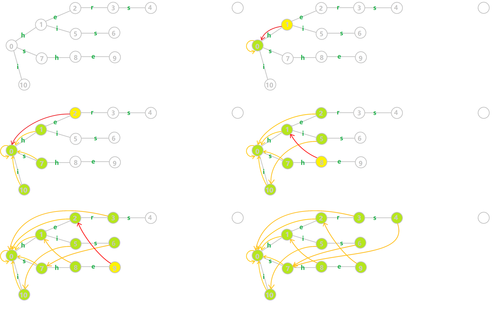
The following GIFs demonstrate the process of constructing fail pointers for a Trie built from the strings \(\mathtt{i}\), \(\mathtt{he}\), \(\mathtt{his}\), \(\mathtt{she}\), \(\mathtt{hers}\):
- Yellow node: the current node \(u\).
- Green node: nodes that have been traversed by BFS.
- Orange edge: fail pointer.
- Red edge: the fail pointer currently being computed.
We focus on constructing the fail pointer for node \(6\):
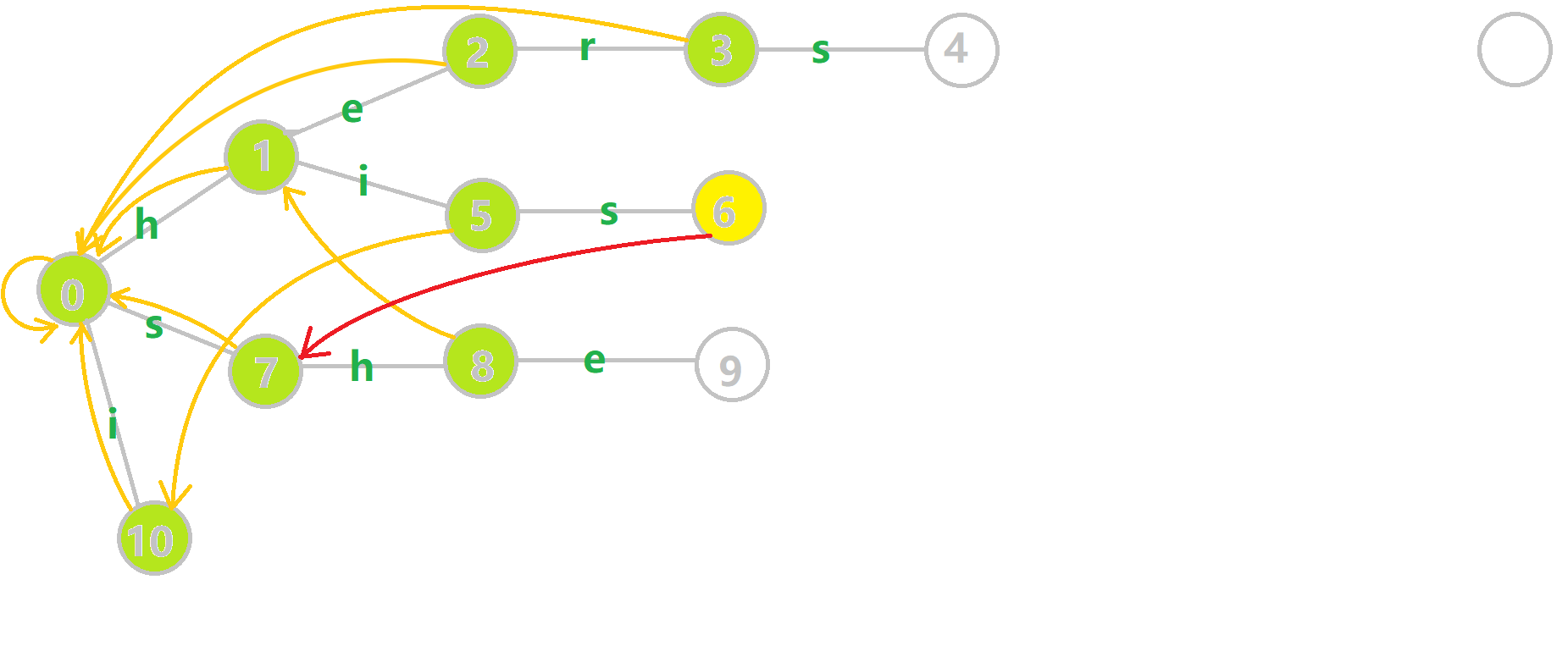
Find the parent node \(5\) of \(6\), \(\operatorname{fail}(5)=10\). However, node \(10\) has no outgoing edge labeled \(\mathtt{s}\); continue jumping to the fail pointer of \(10\), \(\operatorname{fail}(10)=0\). Find that node \(0\) has an outgoing edge labeled \(\mathtt{s}\) pointing to node \(7\); thus \(\operatorname{fail}(6)=7\).
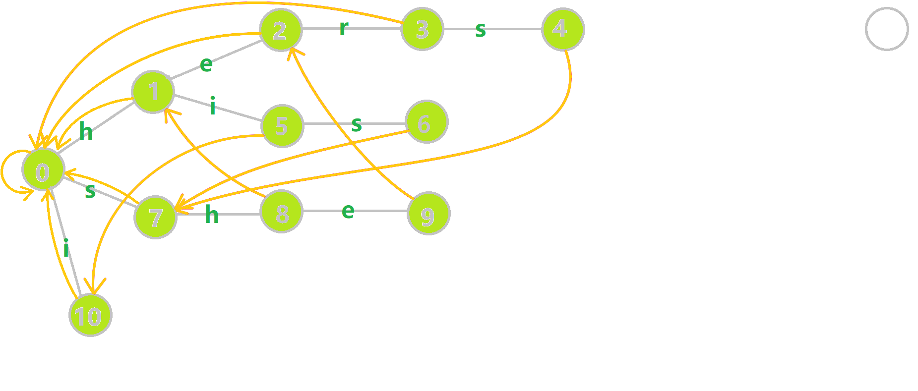
The following figure shows the state after construction is complete:
Trie and Trie Graph
Focus on the build function, which has two goals: constructing fail pointers and building the automaton. Relevant variable definitions are as follows:
tr[u].son[c]: Can be understood in two ways. We can simply think of it as an edge in the Trie, i.e., \(\operatorname{trie}(u, c)\); or as the state (node) reached from state (node) \(u\) by appending a character \(c\), i.e., a state transition function \(\operatorname{trans}(u, c)\). For convenience, we will use the second interpretation in the following text.- Queue
q: used for BFS traversal of the Trie. tr[u].fail: the fail pointer of node \(u\).
Implementation
1 2 3 4 5 6 7 8 9 10 11 12 13 14 15 16 | |
1 2 3 4 5 6 7 8 9 10 11 12 | |
Explanation
The build function enqueues nodes in BFS order, computing fail pointers sequentially. Here, the root node of the Trie is \(0\), and we enqueue all children of the root node. If we enqueued the root node, during the first BFS iteration, the fail pointers of the root's children would be marked as themselves. Therefore, we enqueue the root's children one by one instead of enqueuing the root.
Then BFS begins: each time we take the front node \(u\) from the queue (where \(\operatorname{fail}(u)\) has been computed in previous BFS steps), and iterate over the character set (here \(0 \sim 25\), corresponding to \(\mathtt{a} \sim \mathtt{z}\), i.e., the children of \(u\)):
- If \(\operatorname{trans}(u, c)\) exists, we assign the fail pointer of \(\operatorname{trans}(u, c)\) to \(\operatorname{trans}(\operatorname{fail}(u), c)\). According to the previous description, we should use a
whileloop, repeatedly jumping along fail pointers, checking if a node corresponding to character \(c\) exists, and then assigning it. However, this code simplifies these steps through special handling, which will be explained below; - Otherwise, set \(\operatorname{trans}(u, c)\) to point to the state \(\operatorname{trans}(\operatorname{fail}(u), c)\).
The handling here is that through the else statement, the structure of the Trie is modified, linking non-existent Trie states to the corresponding states of the fail pointer. In the original Trie, each node represents a string \(S\), which is a prefix of some pattern string. After modifying the Trie structure, although many transition relationships are added, the string represented by each node (state) remains unchanged.
And \(\operatorname{trans}(S, c)\) is equivalent to appending a character \(c\) to \(S\) to become another state \(S'\). If \(S'\) exists, it means there is a pattern string prefix that is \(S'\); otherwise, we set \(\operatorname{trans}(S, c)\) to point to \(\operatorname{trans}(\operatorname{fail}(S), c)\). Since the string corresponding to \(\operatorname{fail}(S)\) is a suffix of \(S\), the string corresponding to \(\operatorname{trans}(\operatorname{fail}(S), c)\) is also a suffix of \(S'\).
In other words, when jumping on the Trie, we only jump from \(S\) to \(S'\), which matches an \(S'\); but when jumping on the AC automaton, we jump from \(S\) to a suffix of \(S'\), meaning we match a character \(c\) and then discard part of the prefix of \(S\). Discarding the prefix is obviously matchable. At the same time, if the text string can match \(S\), it can obviously also match suffixes of \(S\), so the fail pointer also discards prefixes. The so-called fail pointer is essentially a suffix set of \(S\).
The child array son of Trie nodes has another simpler interpretation: if a mismatch occurs at position \(u\), we jump to \(\operatorname{fail}(u)\). Note that this may cause us to jump along the fail array multiple times to reach the next matching position. Therefore, we can use son to directly record the next matching position, ensuring the program's time complexity.
The modification to the Trie structure here makes matching transitions more complete. It also compresses the path of fail pointer jumps, turning many fail pointer jumps into a single jump.
Process
Here, several GIFs are used to demonstrate the construction process:
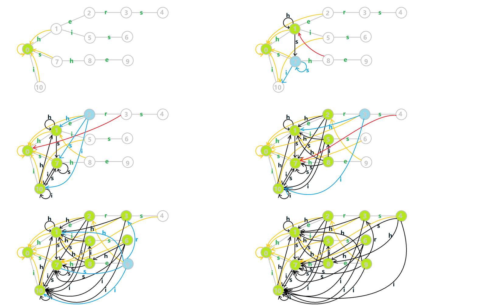
- Blue node: node \(u\) currently being traversed by BFS.
- Blue edge: edges added by the AC automaton modifying the Trie structure under the current node.
- Black edge: edges added by the AC automaton modifying the Trie structure.
- Red edge: fail pointer computed for the current node.
- Yellow edge: fail pointer.
- Gray edge: Trie edges.
It can be observed that numerous intersecting black edges turn the Trie into a Trie graph. Black edges pointing to the root node are omitted in the figure (otherwise it would be more chaotic). Let's focus on the situation when node \(5\) is traversed. We compute the fail pointer for \(\operatorname{trans}(5, \mathtt{s})=6\):
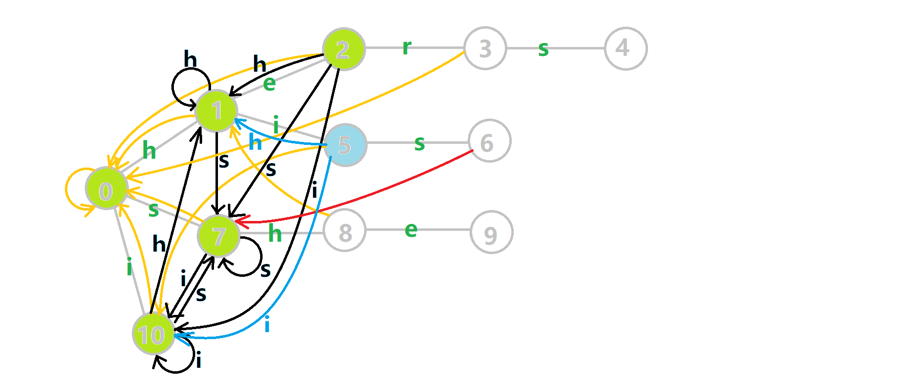
The original strategy is to find the fail pointer, so we jump to \(\operatorname{fail}(5)=10\) and find no outgoing Trie edge labeled \(\mathtt{s}\), then jump to \(\operatorname{fail}(10)=0\), and find \(\operatorname{trie}(0, \mathtt{s})=7\), so \(\operatorname{fail}(6)=7\); but with black and blue edges, after jumping to \(\operatorname{fail}(5)=10\), we directly follow \(\operatorname{trans}(10, \mathtt{s})=7\) to reach node \(7\).
This is what build accomplishes: constructing fail pointers and building the Trie graph. This Trie graph also plays a key role during queries.
Multi-Pattern Matching
Next, analyze the matching function query:
Implementation
1 2 3 4 5 6 7 8 9 10 | |
1 2 3 4 5 6 7 8 9 10 | |
Explanation
Here \(u\) is the current matching node on the Trie, and res is the returned answer. The loop iterates over the matching string, and \(u\) tracks the current character on the Trie. Use fail pointers to find all matching pattern strings and accumulate them into the answer. Then set the occurrence count of matched strings to zero to avoid duplicate counting. As analyzed earlier, the Trie structure is essentially a trans function. After building this function, during string matching, we discard part of the prefix to achieve minimal matching. The fail pointer points to more matching states. Finally, here is a diagram. For the previous automaton:
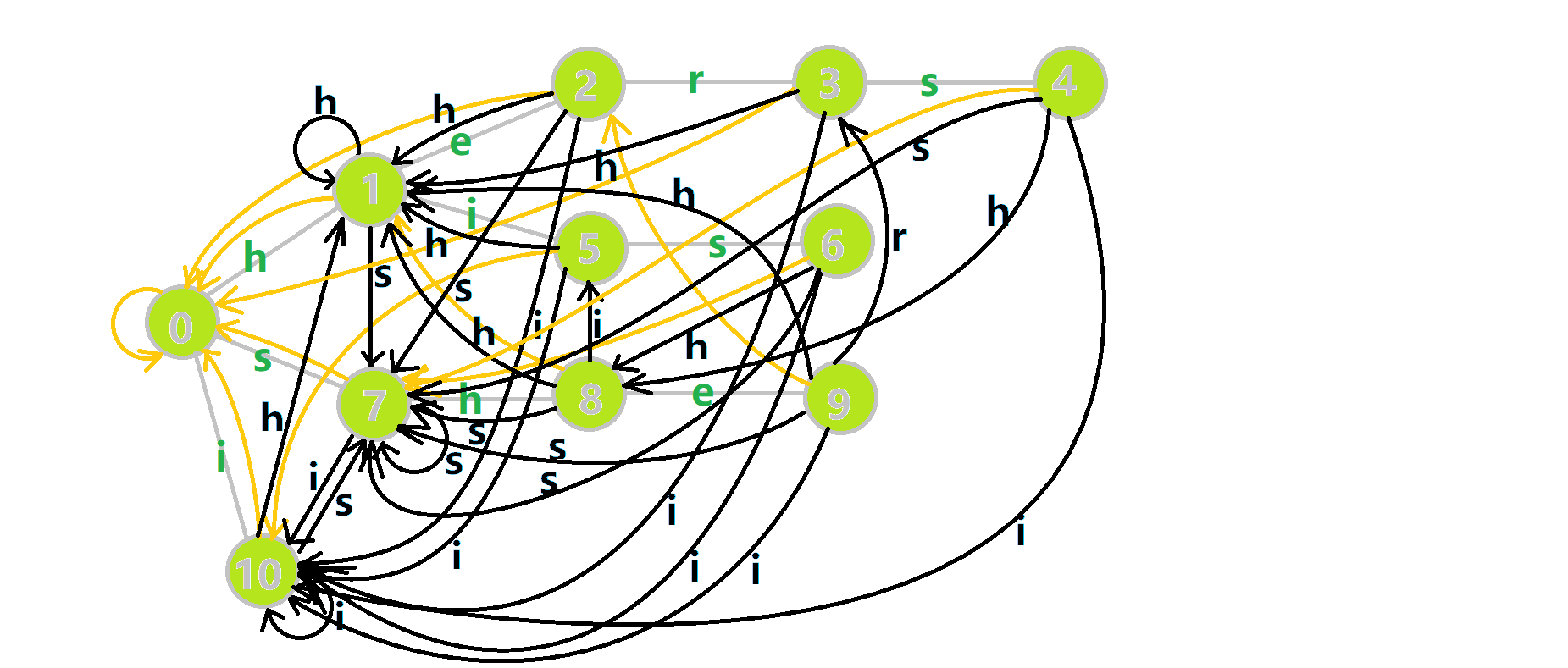
We start from the root node and try to match \(\mathtt{ushersheishis}\). Then the changes of \(p\) will be:
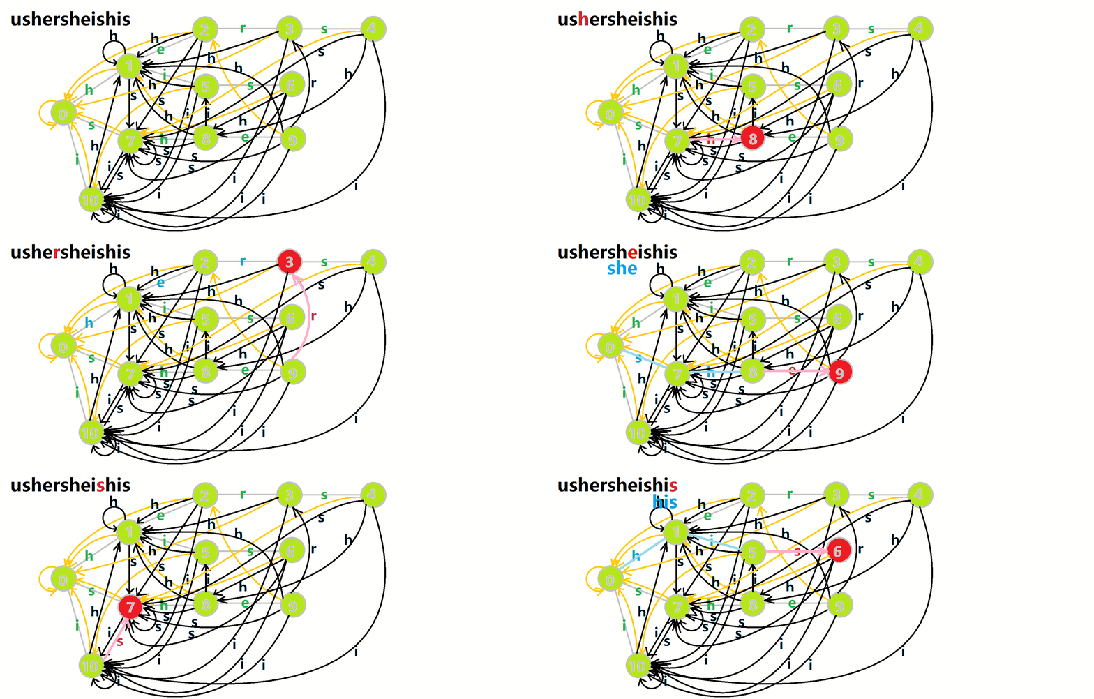
- Red node: node \(p\).
- Pink arrow: jumps of \(p\) on the automaton.
- Blue edge: successfully matched pattern strings.
- Blue node: nodes (states) when jumping along fail pointers.
Efficiency Optimization
Refer to Luogu problem P5357【Template】AC Automaton.
In our AC automaton, each match requires repeatedly jumping along fail edges to find all matches, which is inefficient and may cause timeouts in some problems.
So how can we optimize? First, understand a property of fail pointers: in an AC automaton, if only fail edges are retained, the remaining graph must be a tree.
This is obvious because fail edges cannot form cycles, and the depth is always lower than the current node, thus proven.
Thus, matching in the AC automaton can be transformed into a chain summation problem on the fail tree, and we only need to optimize this part.
Here are two approaches.
Topological Sorting Optimization
Observe that time is mainly wasted on repeatedly jumping along fail pointers. If we can pre-record and sum up at the end, efficiency will improve.
So we perform a topological sort on the fail tree (as an inward tree) to compute the occurrence counts of all pattern strings at once.
The build function, in addition to the original part, includes in-degree statistics to prepare for topological sorting.
Construction
1 2 3 4 5 6 7 8 9 10 11 12 13 14 15 16 17 | |
Then during queries, we only need to mark the ans of found nodes, and finally use topological sorting to compute the answer.
Query
1 2 3 4 5 6 7 8 9 10 11 12 13 14 15 16 17 18 19 20 21 | |
Finally, the main function:
Main Function
1 2 3 4 5 6 7 8 9 | |
Template Problem Luogu P5357「Template」AC Automaton Topological Sorting Optimization Reference Code
1 2 3 4 5 6 7 8 9 10 11 12 13 14 15 16 17 18 19 20 21 22 23 24 25 26 27 28 29 30 31 32 33 34 35 36 37 38 39 40 41 42 43 44 45 46 47 48 49 50 51 52 53 54 55 56 57 58 59 60 61 62 63 64 65 66 67 68 69 70 71 72 73 74 75 76 77 78 79 80 81 82 83 84 85 86 87 88 89 90 91 92 93 94 95 96 97 98 99 100 101 102 103 104 105 106 107 108 109 | |
DFS Optimization
Similar to the topological sorting approach, but we use DFS instead of topological sorting. Essentially, both methods are the same: they both perform subtree summation on the fail tree.
Complete code can be found in Summary Template 3.
DP on AC Automaton
This section uses P2292 [HNOI2004] L Language as an example.
A straightforward idea is to build an AC automaton, perform DP transitions for all substrings along fail pointers on the automaton, and finally take the maximum value as the answer.
The main code is as follows. If unfamiliar with the type definitions in the code, refer to the complete code at the end:
Main Query Code
1 2 3 4 5 6 7 8 9 10 11 12 13 14 15 | |
However, this approach is not linear (because it jumps along each node's fail pointer) and will time out on the second subtask, so optimization is needed.
Looking at the special properties of the problem, we find that all word lengths are at most \(20\), so state compression optimization can be considered.
The current time bottleneck is mainly in jumping along fail pointers. If we can optimize this step to \(O(1)\), we can ensure the entire problem is solved in strictly linear time.
We can store the possible substring lengths within the first \(20\) letters and compress them into states, stored in each child node.
Then in build, we can write:
Constructing Fail Pointers
1 2 3 4 5 6 7 8 9 10 11 12 13 14 15 16 17 18 19 20 21 22 23 24 | |
Then during queries, we can remove the loop for jumping along fail pointers and simplify the code as follows:
Query
1 2 3 4 5 6 7 8 9 10 | |
Our tr[u].stat maintains the set of lengths along the entire fail chain starting from node \(u\) (since the length set is less than \(32\), it does not affect), while st maintains the set of lengths for the first \(32\) bits (due to state compression overflow) of the query string up to the current position.
If the & operation result is non-zero, it means the intersection of the two length sets is non-empty, and we have found a match.
P2292 [HNOI2004] L Language Complete Code
1 2 3 4 5 6 7 8 9 10 11 12 13 14 15 16 17 18 19 20 21 22 23 24 25 26 27 28 29 30 31 32 33 34 35 36 37 38 39 40 41 42 43 44 45 46 47 48 49 50 51 52 53 54 55 56 57 58 59 60 61 62 63 64 65 66 67 68 69 70 71 72 73 74 75 76 77 78 79 80 81 82 83 84 85 86 87 88 89 90 91 92 93 94 95 96 | |
Summary
Time complexity: Let \(|s_i|\) be the length of template strings, \(|S|\) be the length of the text string, and \(|\Sigma|\) be the size of the character set (constant, usually \(26\)). If the trie graph is connected, the time complexity is \(O(\sum|s_i|+n|\Sigma|+|S|)\), where \(n\) is the number of nodes in the AC automaton, which can reach up to \(O(\sum|s_i|)\). If the trie graph is not connected and we avoid traversing empty children when constructing fail pointers, the time complexity is \(O(\sum|s_i|+|S|)\).
Template Problem Luogu P3808 AC Automaton (Simple Version) Reference Code
1 2 3 4 5 6 7 8 9 10 11 12 13 14 15 16 17 18 19 20 21 22 23 24 25 26 27 28 29 30 31 32 33 34 35 36 37 38 39 40 41 42 43 44 45 46 47 48 49 50 51 52 53 54 55 56 57 58 59 60 61 62 63 64 65 66 67 68 69 70 71 72 73 74 75 76 77 78 79 80 81 82 83 84 85 | |
Template Problem Luogu P3796 AC Automaton (Simple Version II) Reference Code
1 2 3 4 5 6 7 8 9 10 11 12 13 14 15 16 17 18 19 20 21 22 23 24 25 26 27 28 29 30 31 32 33 34 35 36 37 38 39 40 41 42 43 44 45 46 47 48 49 50 51 52 53 54 55 56 57 58 59 60 61 62 63 64 65 66 67 68 69 70 71 72 73 74 75 76 77 78 79 80 81 82 83 84 85 86 87 88 89 90 | |
Template Problem Luogu P5357「Template」AC Automaton DFS Optimization Reference Code
1 2 3 4 5 6 7 8 9 10 11 12 13 14 15 16 17 18 19 20 21 22 23 24 25 26 27 28 29 30 31 32 33 34 35 36 37 38 39 40 41 42 43 44 45 46 47 48 49 50 51 52 53 54 55 56 57 58 59 60 61 62 63 64 65 66 67 68 69 70 71 72 73 74 75 76 77 78 79 80 81 82 83 84 85 86 87 88 89 90 91 92 93 94 95 96 97 98 99 100 101 102 103 104 105 | |
本页面最近更新:,更新历史
发现错误?想一起完善? 在 GitHub 上编辑此页!
本页面贡献者:OI-wiki
本页面的全部内容在 CC BY-SA 4.0 和 SATA 协议之条款下提供,附加条款亦可能应用