Partition Tree
Introduction
A Dividing Tree is a data structure used to solve the problem of finding the \(K\)-th largest element in an interval. Its constant factor and difficulty of understanding are much lower than those of a Chairman Tree. At the same time, the Dividing Tree is closely related to the "K-th largest" problem, so it is a data structure based on sorting.
Prerequisite knowledge: Chairman Tree
Process
Building the Tree
Building a Dividing Tree is relatively simple compared to other trees, but still somewhat complex.
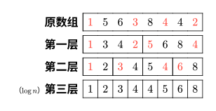
As shown in the figure, each layer has an array that appears unordered. In fact, every number marked in red is to be assigned to the left child. What is the rule for assignment? It is compared with the median of this layer. If it is less than or equal to the median, it goes to the left; otherwise, it goes to the right. However, note that it is not strictly "less than or equal to goes left, otherwise goes right". This is because the median may have duplicates, and it also depends on the parity of \(N\). The following code demonstrates a clever approach; you can refer to the code.
We cannot sort each layer every time; not only would the constant factor be high, but even the theoretical complexity would be unacceptable. Consider finding the median: one sorting operation is enough. Why? For example, to find the median of \(l,r\), it is essentially num[mid] after sorting.
Two key arrays:
tree[log(N),N]: The tree itself, storing all values, with space complexity \(O(n\log n)\). toleft[log(N),n]: The number of elements from 1 to i that go to the left child in each layer. This is a prefix sum and requires some understanding.
Implementation
1 2 3 4 5 6 7 8 9 10 11 12 13 14 15 16 17 18 19 20 21 22 23 24 25 26 27 28 29 30 31 | |
Query
First, let's briefly recall the Chairman Tree. When finding the \(K\)-th smallest element in an interval with a Chairman Tree, we use \(K\) as the benchmark: go left if possible, otherwise go right and subtract the left count. The same principle applies to the Dividing Tree.
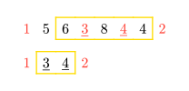
The tricky part of the query is interval narrowing. In the figure below, the query is from \(3\) to \(7\), so the next layer only needs to query \(2\) to \(3\). We define \([\text{left},\text{right}]\) as the narrowed interval (target interval), while \([l,r]\) remains the interval of the current node. Why mark the target interval? Because it is the benchmark for determining whether the answer lies on the left or right.
Implementation
1 2 3 4 5 6 7 8 9 10 11 12 13 14 15 16 | |
Properties
Time complexity: A single query takes \(O(\log n)\), so \(m\) queries take \(O(m\log n)\).
Space complexity: Only \(O(n\log n)\) numbers need to be stored.
Test results: Chairman Tree: \(1482 \text{ms}\), Dividing Tree: \(889 \text{ms}\) (non-recursive, relatively small constant).
Applications of Dividing Tree
Example problem: Luogu P3157[CQOI2011] Dynamic Inversion Pairs
Brief description: Given a permutation of \(n\) elements (\(n\leq 10^5\)), there are m queries (\(m\leq 5\times 10^4\)). After each query, delete a number from the permutation and find the number of inversion pairs in the permutation after deletion.
This problem can be solved using CDQ in \(\Theta(n\log^2n)\) time and \(\Theta(n)\) space, and CDQ also has excellent constant factors.
If the problem is changed to force online queries, a common solution uses a Fenwick Tree + Chairman Tree (tree of trees), with time complexity \(\Theta(n\log^2n)\), space complexity \(\Theta(n\log^2n)\), and a relatively large constant, but it can still pass this problem.
Using a Dividing Tree, this problem can be solved online in \(\Theta(n\log^2n)\) time and \(\Theta(n\log n)\) space, with a much smaller constant compared to the tree-of-trees solution (roughly comparable to CDQ).
Note
For programming convenience, this article divides large arrays into two smaller arrays based on the median of positions. That is, the Dividing Tree here is equivalent to the process of merge sort, not quicksort. The top layer is a sorted array, and the bottom layer is the original array.
For each node in the Dividing Tree, we call it a right node if and only if it will be assigned to the right child in the next layer, i.e., numbers with relatively later positions in the original array. Similarly, we can define left nodes. If the top layer is sorted during construction, similar to using merge sort to count inversion pairs, we can find that the number of inversion pairs in an array is the sum of the number of right nodes before each left node.
Now consider deletion operations. Deleting a left node reduces the total inversion pairs by the number of right nodes before it, while deleting a right node reduces the inversion pairs by the number of left nodes after it. Thus, we can dynamically maintain "the number of right nodes before each left node" and "the number of left nodes after each right node". This can be easily maintained using a Fenwick Tree.
Note that when using a Fenwick Tree for maintenance, we can only compute contributions within the same block of the Dividing Tree and cannot cross block boundaries. There is a clever way to handle this with a Fenwick Tree.
Consider that the index range of each block in the Dividing Tree must be of the form \([c\times 2^k+1,(c+1)\times 2^k]\), as listed below (since the code does not involve processing the bottom layer of the Dividing Tree, only enumerating down to the second-to-last layer):
1 2 3 4 | |
Recall the principle of Fenwick Tree: when jumping upward, we do x += lowbit(x). If we can ensure not to jump out of the block while jumping upward, we can guarantee that only elements within the block are affected. Similarly for upward queries.
To ensure not to jump out of the block while jumping upward, it is sufficient to ensure that \(lowbit(x)<2^{lev}\) during the jump.
Downward jumps are handled completely differently. If the indices of each block are represented using 0-index notation, they are of the form \([c\times 2^k,(c+1)\times 2^k)\). Then, simply right-shift an index value by k to determine which block it belongs to. During downward jumps, continuously check whether the jump crosses block boundaries.
Note that the maximum index accessed by the Fenwick Tree implemented this way is the nearest power of two to n, so the array size cannot be set to n.
Since modifications are required in \(\log n\) layers, and the time complexity for modification at layer \(k\) is \(\Theta(k)\), the final time complexity is \(\Theta(n\log n+m\log^2n)\).
Attached code:
1 2 3 4 5 6 7 8 9 10 11 12 13 14 15 16 17 18 19 20 21 22 23 24 25 26 27 28 29 30 31 32 33 34 35 36 37 38 39 40 41 42 43 44 45 46 47 48 49 50 51 52 53 54 55 56 57 58 59 60 61 62 63 64 65 66 67 68 69 70 71 72 73 74 75 76 77 78 79 80 81 82 83 84 85 86 87 88 89 90 91 92 93 94 95 96 97 98 99 100 101 102 103 104 105 106 107 108 109 110 111 112 113 114 115 116 | |
Afterword
Reference blog: Link.
本页面最近更新:,更新历史
发现错误?想一起完善? 在 GitHub 上编辑此页!
本页面贡献者:OI-wiki
本页面的全部内容在 CC BY-SA 4.0 和 SATA 协议之条款下提供,附加条款亦可能应用