WQS Binary Search
Introduction
This article introduces the method of using WQS binary search to optimize dynamic programming problems. In various literature, it is also commonly referred to as weighted binary search, convex optimization DP, convex complete monotonicity DP, Lagrange multiplier method, etc., and is known abroad as the Aliens Trick. It was first summarized by Wang Qinshi in the article "A Brief Analysis of a Class of Binary Methods".
WQS binary search is typically used to solve optimization problems with quantity constraints, where direct solution is costly; however, once this constraint is removed, the problem itself becomes much easier to solve.
For example, suppose the problem is to select \( m \) items from \( n \) items and optimize a relatively complex objective function. If we denote the optimal value of the objective function when selecting \( j \) items from the first \( i \) items as \( f(i,j) \), then the answer to the original problem is \( f(n,m) \). In such problems, the state transition equation is usually two-dimensional. Directly implementing this state transition equation results in a time complexity of \( O(nm) \), which is often unacceptable.
Further assume that the optimization problem without quantity constraints is easy to solve. However, the optimal number of items selected may not satisfy the original problem's quantity constraint. Suppose too many items are selected. Then, we can consider adding a fixed penalty \( k \) (the "weight" in "weighted binary search") to each selected item when solving the unconstrained optimization problem. Depending on the value of \( k \), the optimal number of items selected will vary; moreover, as \( k \) changes, the optimal number of items selected changes monotonically. Therefore, by binary searching, we can find a \( k \) such that the optimal number of items selected is exactly \( m \). Suppose the optimal value of the objective function at this point is \( f_k(n) \); then, by eliminating the value loss caused by the additional penalty, we can obtain the answer to the original problem: \( f(n,m)=f_k(n)+km \). Assuming the complexity of solving the penalized problem once is \( O(T(n)) \), the overall complexity of the algorithm is reduced to \( O(T(n)\log L) \), where \( O(\log L) \) is the number of binary search steps needed for \( k \).
This is the basic idea of WQS binary search. However, for this idea to work, it is necessary that \( f(n,m) \) is convex with respect to \( m \). Otherwise, there may not exist an additional penalty \( k \) that makes the optimal number exactly \( m \). This is also why this DP optimization method is often called "convex optimization DP" or "convex complete monotonicity DP".
Traditional Method
Let the non-empty set \( X \) be the (finite) decision space, \( f:X\rightarrow\mathbf R \) be the objective function, and let there be another function \( g:X\rightarrow\mathbf R^d \) for imposing constraints. The problem to be solved can be viewed as computing the value function \( v(y) \) of the following optimization problem at a certain point:
For example, for the quantity-constrained problem mentioned earlier, \( X \) can be understood as the family of all subsets of the item set, \( x\in X \) is a single subset, \( f(x) \) is the value function of a single subset, and \( g(x) \) is the number of elements in subset \( x \). Of course, \( g(x) \) is not limited to quantity constraints; later sections provide examples of more general constraints.
Convention
For convenience, this article only discusses problems of minimizing the objective function. Problems of maximizing the objective function are similar, except that the (lower) convex functions in this article should be replaced with concave functions (or upper convex functions). Alternatively, by adding a negative sign, the problem of maximizing the objective function can be transformed into minimizing its negative.
Geometric Intuition
Since most problems encountered in algorithmic competitions are combinatorial optimization problems, the decision space \( X \) usually lacks a nice structure. Therefore, we can instead consider the set
The traditional method mainly addresses the case where \( d=1 \), i.e., there is only one constraint. The following figure provides a possible illustration of the point set \( \mathcal D \) in this case.
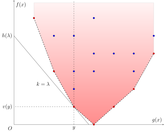
The red and blue points in the figure are the set \( \mathcal D \) obtained by projecting all possible choices in \( X \) onto the plane \( (g(x),f(x)) \). Thus, what the original problem requires is the minimum ordinate \( v(y) \) among those points with abscissa \( y \). As \( y \) varies, all such points \( (y,v(y)) \) form the set of red points in the figure.
To find the ordinate of point \( (y,v(y)) \), consider using a line with slope \( \lambda\in\mathbf R \) to cut the set \( \mathcal D \). As shown in the figure, when the slope of the line is chosen appropriately, the line passing through point \( (y,v(y)) \) is the one among all lines with slope \( \lambda \) that pass through points in set \( \mathcal D \) and have the smallest intercept \( f(x)-\lambda g(x) \). Denote this minimum value as
Then, since \( (y,v(y)) \) also lies on this line, we can obtain the solution to the original problem:
Assume that for all reasonable ranges of \( \lambda \), the function \( h(\lambda) \) above is easy to compute. This is often true in algorithmic competitions because it removes the constraints of the original problem. Then, the two most important questions now are:
- Does there exist such a line slope \( \lambda \) such that its minimum intercept is exactly achieved at point \( (y,v(y)) \), and
- If it exists, how to find such a slope \( \lambda \).
The first question is relatively easy to answer. Because when the line slope \( \lambda \) changes, the set cut out by all these lines (i.e., the intersection of their upper half-planes) must be a convex set. Therefore, these lines can pass through a point if and only if that point lies on the lower convex hull of this convex set. This is equivalent to saying that the function \( v(y) \) is a convex function.
The second question is more delicate. Since the abscissa of the desired point is known to be \( y \), a natural idea is, when computing \( h(\lambda) \), to also find the value of the constraint function \( g(x) \) at the current optimal solution \( x_\lambda \). For example, in the earlier example, when solving the penalized problem, we can record the number of items selected when the penalized objective function achieves its optimal value. Then, compare \( g(x_\lambda) \) with the desired \( y \), and adjust the value of \( \lambda \) for the next computation accordingly. This is the most traditional WQS binary search method.
To summarize, the basic flow of traditional WQS binary search is as follows:
- Initially, select a reasonable interval for \( \lambda \);
- Choose a \( \lambda \) within the current interval;
- Solve the penalized problem \( h(\lambda)=\min_{x\in X}f(x)-\lambda g(x) \), and record the value \( g(x_\lambda) \) of \( g(x) \) at its optimal solution \( x_\lambda \);
- If \( g(x_\lambda)=y \), then the optimal value of the original problem is \( v(y)=h(\lambda)+\lambda y \), and the algorithm ends directly;
- Otherwise, adjust the interval of \( \lambda \) based on the relationship between \( g(x_\lambda) \) and \( y \), and return to step 2.
This basic flow is sufficient to solve some problems, but it is not perfect. Next, this article will discuss improvements to this basic flow.
Handling Collinear Cases
When applying the basic flow, the first problem encountered is that collinear cases cannot be handled correctly.
If there are three or more red points on the lower convex hull of point set \( \mathcal D \) that are collinear, then in the basic flow above, it may not be possible to correctly determine the relationship between \( g(x_\lambda) \) and \( y \). For example, let the abscissas of three collinear red points be \( y_1, y_2, y_3 \), and the slope of their common line be \( \lambda^* \). Then, to correctly solve \( v(y_2) \), we must ensure that when the algorithm terminates, the last computed problem is \( h(\lambda^*) \), because \( \lambda^* \) is the only slope for which the line minimizing the intercept can pass through point \( (y_2,v(y_2)) \). However, during the solution of \( h(\lambda^*) \), the recorded \( g(x_{\lambda^*}) \) could be any of \( y_1, y_2, y_3 \). If the recorded \( g(x_{\lambda^*}) \) is not equal to \( y_2 \), the algorithm will incorrectly continue and adjust the interval of \( \lambda \) in a direction away from \( y_2 \), eventually yielding an incorrect result.
To handle collinear cases, one approach is to always make the recorded \( g(x_\lambda) \) corresponding to the optimal solution \( x_\lambda \) as large as possible (or as small as possible). At the same time, change the termination condition in the binary search from finding a \( \lambda \) that exactly satisfies \( g(x_\lambda)=y \) to finding the smallest (or largest) \( \lambda \) that satisfies \( g(x_\lambda)\ge y \) (or \( g(x_\lambda)\le y \)). In the example from the previous paragraph, this is equivalent to outputting \( g(x_{\lambda^*}) \) as \( y_3 \) when computing problem \( h(\lambda^*) \). This ensures that when the algorithm terminates, the last computed problem is \( h(\lambda^*) \). When implementing this method, note that the final output is not \( h(\lambda)+\lambda g(x_{\lambda}) \) but \( h(\lambda)+\lambda y \), because the recorded \( g(x_\lambda) \) may not equal the actual constraint \( y \).
Another approach is real-number binary search. If the numbers involved in the problem are all integers, clearly the slope in WQS binary search is also an integer. Introducing real numbers in binary search is to ensure that if the correct option \( \lambda^* \) is incorrectly excluded, it can be adjusted back via the fractional part, eventually approaching the correct answer \( \lambda^* \). For example, in the above case, if when computing problem \( h(\lambda^*) \), the recorded \( g(x_{\lambda^*}) \) is \( y_1 \), which is less than the desired \( y_2 \), then the algorithm will turn to consider the interval \( (\lambda^*,\lambda_r] \), where \( \lambda_r \) is the right endpoint of the interval containing \( \lambda \). For integer cases, this interval should actually be written as \( [\lambda_*+1,\lambda_r] \), which excludes the possibility of approaching the correct answer \( \lambda^* \) in subsequent steps. However, with real-number binary search, the considered interval is still \( (\lambda^*,\lambda_r] \), and for \( \lambda \) in this interval, the recorded \( g(x_\lambda) \) when solving \( h(\lambda) \) is always not less than \( y_3 \), thus strictly greater than \( y_2 \). Therefore, as the algorithm continues, the right half-interval is continuously discarded, so the final range of \( \lambda \) can be guaranteed to be near \( \lambda^* \). Of course, since we know the desired slope is an integer, the precision when real-number binary search terminates need not be too high; it only needs to ensure that the binary search interval contains only one integer, which is the desired \( \lambda^* \).
After correctly handling collinear cases, WQS binary search is sufficient to solve most WQS binary search problems encountered in algorithmic competitions. However, this method still has some shortcomings: it cannot handle cases where \( g(x_\lambda) \) is difficult to record, nor can it handle cases where multiple points are coplanar in high-dimensional WQS binary search. This article will further examine the properties of the optimization problem \( v(y) \) and propose more general handling methods.
Dual Method
This section introduces an implementation method for WQS binary search that only requires efficiently computing
for all \( \lambda\in\mathbf R^d \), and that the original problem's optimal value function \( v(y) \) is a convex function with respect to \( y\in\mathbf R^d \)[^high-d-convex]. In a nutshell, this section will prove that the original problem's value function \( v(y) \) equals the optimal value of its dual problem:
and the dual problem's objective function is a concave function with respect to \( \lambda\in\mathbf R^d \), hence unimodal, which can be efficiently solved via the ternary search method or the golden section search method, with complexity still \( O(T(n)\log^d L) \). This completely solves the issues that may arise when recording the value of \( g(x_\lambda) \) in the traditional WQS binary search method, while also allowing the application of WQS binary search ideas to high-dimensional cases.
Additionally, this section explains that the range of \( g(x_\lambda) \) can be obtained from \( h(\lambda) \) without needing to record it additionally when solving \( h(\lambda) \). For example, for the case where \( d=1 \) and the problem involves only integers, it can be proven that the range of \( g(x_\lambda) \) is exactly
This actually provides another method for solving collinear problems for problems that must adopt the binary search flow described earlier.
Next, this section will use convex analysis theory to prove these conclusions. For specific applications of these methods, refer to the Examples section.
Lagrange Duality
Consider solving the problem using the Lagrange multiplier method. Introduce Lagrange multipliers \( \lambda\in\mathbf R^d \); then the Lagrangian can be written as
Because as long as any component of \( g(x)-y \) is non-zero, the corresponding component of \( \lambda \) can be made to approach (positive or negative) infinity, we have
This shows that the original problem can be written as
Swapping the two extremization operations yields its dual problem:
We will now show that under the condition that \( v(y) \) is a convex function with respect to \( y \), strong duality holds, i.e., \( v^\star(y)=v(y) \).
Convex Conjugate
To show strong duality holds, we need to introduce the concept of the convex conjugate.
Convex Conjugate
For a function \( f:\mathbf R^d\rightarrow\mathbf R\cup\{\pm\infty\} \), its convex conjugate, or Legendre–Fenchel transformation, is the function
From the perspective of variable \( x^* \), \( f^*(x^*) \) is the supremum of a family of linear functions, so it must be a convex function on \( \mathbf R^d \).
「Slope Vector」 and 「Intercept」 of a Hyperplane
The equations of hyperplanes in the vector space \( \mathbf R^{d+1} \) discussed in this article all have the form
That is, this article will not involve hyperplanes parallel to the \( y \)-axis. For convenience, this article informally refers to \( k \) as the "slope vector" of the hyperplane and \( b \) as its "intercept". Writing this hyperplane equation in a more standard form gives
One of its normal vectors is \( (k,-1) \). Therefore, the so-called slope vector is actually the first \( d \) components of the normal vector obtained by normalizing the hyperplane's normal vector such that its last component equals \( -1 \).
Geometrically, the convex conjugate of a function \( f(x) \) describes that for all hyperplanes with slope vector \( x^* \) that intersect the epigraph of \( f(x) \)
the minimum intercept \( f(x)-x^*\cdot x \) is \( -f^*(x^*) \). In other words, the function \( f(x) \) always lies above the hyperplane \( y = x^*\cdot x-f^*(x^*) \) and is tangent to this plane at point \( (x_0,f(x_0)) \); of course, there may be other points of tangency. Such a hyperplane is called a supporting hyperplane of \( f(x) \) at \( x_0 \). The intercept of a supporting hyperplane of \( f(x) \) is uniquely determined by its slope vector; the convex conjugate provides this mapping from slope vector to intercept.
Minimizing \( f(x)-\lambda\cdot g(x) \) over set \( X \) is equivalent to minimizing \( v(y)-\lambda\cdot y \) over the set \( \{(y,v(y))\} \):
Therefore, we have
This shows that \( h(\lambda) \) is a concave function with respect to \( \lambda\in\mathbf R^d \). Furthermore,
That is, the dual problem's value function \( v^{\star}(y) \) is the biconjugate of the original problem's value function \( v(y) \), also called the double conjugate.
Thus, the problem reduces to: what kind of function \( v(y) \) satisfies that its double conjugate equals itself? The answer to this question is given by the following theorem:
Theorem (Fenchel–Moreau)
For a function \( f:\mathbf R^d\rightarrow\mathbf R\cup\{\pm\infty\} \), its double conjugate equals itself, i.e., \( f^{**}=f \), if and only if one of the following three conditions holds:
- \( f(x) \) is a proper convex function and lower semicontinuous,
- \( f(x)\equiv+\infty \), or
- \( f(x)\equiv-\infty \).
Proof
A function is proper if and only if it never takes the value \( -\infty \) and does not always take the value \( +\infty \).
For improper functions, it can be verified that \( f(x)\equiv+\infty \) and \( f(x)\equiv-\infty \) are conjugates of each other. Apart from these, if \( f(x) \) takes \( -\infty \) at any point, then necessarily \( f^*(x^*)\equiv+\infty \). So the only improper functions satisfying \( f^{**}=f \) are these two cases. The following discussion is limited to proper functions. For proper functions, the condition of being lower semicontinuous and convex is equivalent to its epigraph being a closed convex set.
The necessity of this condition is easy. Because \( f=f^{**} \) is the convex conjugate of \( f^* \), as the supremum of a family of linear functions, its epigraph must be the intersection of a family of closed convex sets, so it must be a closed convex set. This shows that any proper function satisfying \( f^{**}=f \) must be lower semicontinuous and convex.
Conversely, these conditions are also sufficient. Like other strong duality theorems, the proof can be divided into two steps.
First, show that weak duality holds, i.e., \( f(x)\ge f^{**}(x) \). By the definition of convex conjugate, for all \( x,x^*\in\mathbf R^d \), we have
This implies that for all \( x,x^*\in\mathbf R^d \), we also have
Taking the supremum over \( x^* \) on the right-hand side of the inequality gives \( f(x)\ge f^{**}(x) \).
Second, use the hyperplane separation theorem to show \( f(x)\le f^{**}(x) \). Suppose not; there exists \( x_0\in\mathbf R^d \) such that \( f(x_0)>f^{**}(x_0) \). Because the epigraph \( \operatorname{epi}(f) \) of \( f(x) \) is a closed convex set, and the singleton set \( \{(x_0,f^{**}(x_0))\} \) is a compact convex set, by the hyperplane separation theorem, there exist \( (\lambda,t)\in\mathbf R^d\times\mathbf R \) and \( \alpha\in\mathbf R \) such that for all \( x\in\operatorname{dom} f:=\{x\in\mathbf R^d:f(x)<+\infty\} \) and all \( y\ge f(x) \), we have
Because \( y \) can be chosen arbitrarily large, we must have \( t\ge 0 \). This can be divided into two cases.
First, consider the case \( t>0 \). Dividing all parts of the inequality by \( t \), and setting \( \lambda'=t^{-1}\lambda \) and \( \alpha'=t^{-1}\alpha \), we get
For all \( x\in\operatorname{dom} f \), letting \( y=f(x) \), we have
Therefore, taking the supremum over \( x \) on the right-hand side of the inequality, we have
Then,
This contradiction shows that the case \( t>0 \) cannot hold.
Finally, consider the case \( t=0 \). In fact, we will show that it can be transformed into the case \( t>0 \) via perturbation. Choose any \( \lambda_0\in\operatorname{dom}f^* \). By the definition of convex conjugate, for any \( x\in\operatorname{dom}f \) and \( y\ge f(x) \), we have
Therefore, for any \( \varepsilon>0 \), we have
At the same time, because \( \alpha<\lambda\cdot x_0 \), for sufficiently small \( \varepsilon>0 \), we also have
Thus, if we set \( \lambda'=\lambda+\varepsilon\lambda_0 \), \( t'=\varepsilon \), and \( \alpha'=\alpha+\varepsilon f^*(\lambda_0) \), then we have
This returns to the previous case, which still leads to a contradiction.
This contradiction shows that there does not exist a point \( x_0\in\mathbf R^d \) satisfying \( f(x_0)>f^{**}(x_0) \). Hence, we always have \( f(x_0)\le f^{**}(x_0) \).
Combining the results of these two steps, we obtain \( f^{**}(x)=f(x) \).
Therefore, strong duality holds if and only if \( v(y) \) is a convex function with respect to \( y\in\mathbf R^d \)[^other-conditions].
Subgradient
The previous section showed that the value function \( h(\lambda) \) of the penalized problem is the negative of the convex conjugate of the original problem's value function \( v(y) \). Because the definition of the convex conjugate is essentially a parametric optimization problem, it also satisfies conclusions similar to the envelope theorem. However, since convex functions are not everywhere differentiable, we first need to generalize the definition of derivative to convex functions. This leads to the concept of subgradient.
Subgradient
For a convex function \( f:\mathbf R^d\rightarrow\mathbf R\cup\{\pm\infty\} \) and \( x_0\in\operatorname{dom}f \), if a vector \( x^*\in\mathbf R^d \) satisfies for any \( x\in\mathbf R^d \),
then \( x^* \) is called a subgradient of \( f(x) \) at \( x_0 \). The set of all subgradients of \( f(x) \) at \( x_0 \) is called its subdifferential at that point, denoted \( \partial f(x_0) \).
Geometrically, the subdifferential of a convex function \( f(x) \) at \( x_0 \) is the set of slope vectors of all its supporting hyperplanes at that point. For the one-dimensional case, the subdifferential
where \( \partial_-f(x_0) \) and \( \partial_+f(x_0) \) are the left and right derivatives of \( f(x) \) at \( x_0 \), respectively. Furthermore, for a convex function \( f:\mathbf Z\rightarrow\mathbf R\cup\{\pm\infty\} \) extended from integers, its left and right derivatives at integer point \( x=k \) are the left and right first differences:
Clearly, a convex function \( f(x) \) is differentiable at point \( x_0 \) if and only if its subdifferential \( \partial f(x_0) \) is a singleton.
Because the convex conjugate provides the mapping from the slope vector of a supporting hyperplane to its intercept, we can use the convex conjugate to determine whether a slope vector \( x^* \) is a subgradient of a convex function \( f(x) \) at a given point \( x \).
Theorem (Convex Conjugate and Subgradient)
For a proper convex function \( f:\mathbf R^d\rightarrow\mathbf R \) and any \( x,x^*\in\mathbf R^d \), we have
Furthermore, if \( f \) is also lower semicontinuous, then both conditions are equivalent to \( x\in\partial f^*(x^*) \).
Proof
By the definition of subgradient, \( x^*\in\partial f(x) \) if and only if
This is equivalent to
Which is equivalent to
However, by the definition of convex conjugate, we always have
Therefore, the greater-than-or-equal sign in the previous expression is actually equivalent to equality, which is equivalent to
This completes the first part of the proof.
For the case where \( f \) is a lower semicontinuous proper convex function, by the Fenchel–Moreau theorem, we have \( f^{**}=f \). Therefore, these two conditions are equivalent to
Applying the first part's conclusion again, they are also equivalent to \( x\in\partial f^*(x^*) \).
This conclusion shows that if \( f^{**}=f \), then the subdifferential \( \partial f^{*}(x^*) \) of the convex conjugate \( f^* \) at \( x^* \) is exactly the set of \( x \)-components of the intersection points of the supporting hyperplane with slope vector \( x^* \) and the epigraph \( \operatorname{epi}f \).
Corollary
For a lower semicontinuous proper convex function \( f:\mathbf R^d\rightarrow\mathbf R \) and any \( x,x^*\in\mathbf R^d \), we have
Proof
Below, we prove the second equality. The proof of the first is similar.
By the definition of convex conjugate,
so
if and only if \( f^*(x^*) = x^*\cdot x - f(x) \), and this equality holds if and only if \( x\in\partial f^*(x^*) \). This proves the two sets are equal.
Applying this to the context of this article, this conclusion shows that when solving the problem
the values of the constraint function \( g(x) \) on the optimal decision set are exactly \( \partial(-h(\lambda)) \). For the case \( d=1 \) and the problem involves only integers, this set is the interval
For consecutive integers \( \lambda \), these intervals connect end to end, so if used for binary search, only one endpoint needs to be computed.
Convexity Proof
The prerequisite for applying WQS binary search is the convexity of the value function. In algorithmic competitions, convexity can be conjectured via methods like brute-force enumeration or intuitive understanding. However, rigorously proving convexity is often not easy. This section, combined with the following classic problem, introduces common methods for proving convexity in algorithmic competitions.
Tree Planting Problem
There are \( n \) tree pits, and \( m \) trees need to be planted. Trees cannot be planted in two adjacent pits. Given a sequence \( \{a_i\} \) of length \( n \), representing the profit of planting a tree in each pit (profits can be positive or negative). Find the maximum possible total profit after planting these \( m \) trees.
In short, it is the problem of finding a maximum weight independent set of size \( m \) on a chain of length \( n \).
These methods can be roughly divided into four categories:
- Reduce to the convexity of the value function of a convex optimization problem (including linear programming, etc.), which includes methods like constructing a minimum cost flow model;
- Use the state transition equation to inductively prove convexity, possibly using some convexity-preserving transformations;
- For interval partitioning problems, verify that the cost function of each interval satisfies the quadrangle inequality;
- Finally, for special problems, convexity can also be directly shown via exchange arguments.
These proof methods themselves are often connected to some solution approach for the problem.
Reduction to Parametric Convex Optimization
Consider a parametric convex optimization problem of the form:
Here, the objective function \( f:\mathbf R^n\times\mathbf R^d\rightarrow\mathbf R\cup\{\pm\infty\} \) is convex in \( x\in\mathbf R^m \) for each \( y\in\mathbf R^d \), and the feasible region mapping \( \mathcal D:\mathbf R^d\rightarrow \mathcal P(\mathbf R^m) \) is a set-valued function on \( \mathbf R^d \), and for each \( y\in\mathbf R^d \), the set \( \mathcal D(y) \) is convex. These conditions ensure that for any parameter \( y\in\mathbf R^d \), this is a convex optimization problem.
Theorem
Assume the above parametric convex optimization problem satisfies the following conditions:
- The objective function \( f(x,y) \) is convex in \( (x,y) \);
- The graph of the feasible region mapping \( y\mapsto\mathcal D(y) \), \( \{(x,y):x\in\mathcal D(y)\} \), is a convex set.
If for any \( y\in\mathbf R^d \), we have \( v(y)>-\infty \), then the value function \( v(y) \) is a proper convex function in \( y \).
Proof
For any \( y_1,y_2\in\mathbf R^d \) and \( \alpha\in(0,1) \), we need to prove
If \( v(y_1)=+\infty \) or ( v(y_2
本页面最近更新:,更新历史
发现错误?想一起完善? 在 GitHub 上编辑此页!
本页面贡献者:OI-wiki
本页面的全部内容在 CC BY-SA 4.0 和 SATA 协议之条款下提供,附加条款亦可能应用