Prüfer Sequence
Note
This article is translated from e-maxx Prüfer Code. Additionally, note that the original article labels nodes starting from \(0\), while this article follows the common convention of labeling from \(1\).
This article introduces the Prüfer sequence (Prüfer code), a method to uniquely represent a labeled tree using an integer sequence.
Using the Prüfer sequence, one can prove Cayley's formula. We will also explain how to calculate the number of ways to add edges to make a graph connected.
Note: We do not consider trees with \(1\) node.
Prüfer Sequence
Introduction
The Prüfer sequence can represent a labeled tree with \(n\) nodes using \(n-2\) integers from \([1,n]\). You can also think of it as a bijection between spanning trees of a complete graph and sequences. It is commonly used in combinatorial counting problems.
Heinz Prüfer invented this sequence in 1918 to prove Cayley's formula.
Constructing the Prüfer Sequence from a Tree
The Prüfer sequence is constructed as follows: repeatedly remove the leaf node with the smallest label, and record the label of the node it was connected to. After \(n-2\) repetitions, only two nodes remain, and the algorithm ends.
Clearly, using a heap can achieve \(O(n\log n)\) complexity.
Implementation
1 2 3 4 5 6 7 8 9 10 11 12 13 14 15 16 17 18 19 20 21 22 23 24 25 26 | |
1 2 3 4 5 6 7 8 9 10 11 12 13 14 15 16 17 18 19 20 21 22 23 24 25 26 | |
For example, here is the construction process of the Prüfer sequence for a tree with 7 nodes:
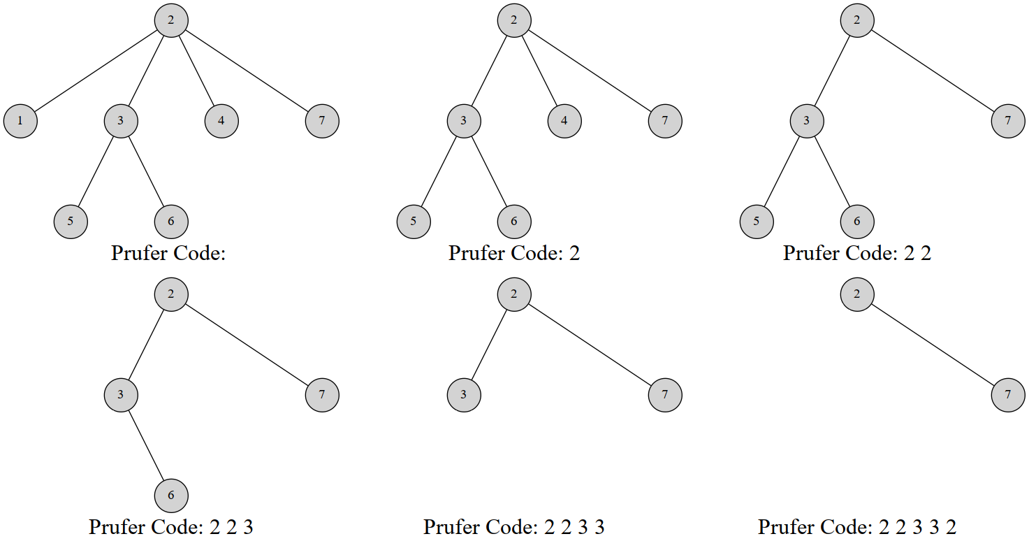
The final sequence is \(2,2,3,3,2\).
Of course, there is also a linear construction algorithm.
Linear Construction Algorithm for Prüfer Sequence
The essence of the linear construction is to maintain a pointer pointing to the node we are about to delete. First, note that the number of leaf nodes is non-strictly decreasing; removing a leaf node either keeps the total number of leaves the same or reduces it by 1.
Thus, we consider the following process: maintain a pointer \(p\). Initially, \(p\) points to the leaf node with the smallest label. We also maintain the degree of each node to know whether new leaf nodes are generated when deleting a node. The operations are as follows:
- Delete the node pointed to by \(p\), and check if a new leaf node is generated.
- If a new leaf node is generated, denote its label as \(x\), and compare \(p\) and \(x\). If \(x>p\), then do nothing; otherwise, immediately delete \(x\), then check if deleting \(x\) generates a new leaf node, repeating step \(2\) until no new node is generated or the new node's label \(>p\).
- Increment the pointer \(p\) until it encounters an undeleted leaf node.
Correctness
After repeating the above operations \(n-2\) times, the sequence is constructed. Now consider the correctness of the algorithm.
\(p\) is the current smallest leaf node. If deleting \(p\) does not generate a leaf node, we must find the next leaf node; if it generates a leaf node \(x\):
- If \(x>p\), then \(p\) will eventually scan to it anyway, so no operation is needed;
- If \(x<p\), because \(p\) was originally the smallest, and \(x\) is even smaller than \(p\), \(x\) is now the current smallest leaf node, so it should be deleted first. Deleting \(x\) continues this consideration until there is no smaller leaf node.
Analyzing the algorithm's complexity, each edge is visited at most once (when decrementing degrees), and the pointer traverses each node at most once, so the complexity is \(O(n)\).
Implementation
1 2 3 4 5 6 7 8 9 10 11 12 13 14 15 16 17 18 19 20 21 22 23 24 25 26 27 28 29 30 31 32 33 34 35 36 37 | |
1 2 3 4 5 6 7 8 9 10 11 12 13 14 15 16 17 18 19 20 21 22 23 24 25 26 27 28 29 30 31 32 33 34 35 36 37 38 | |
Properties of the Prüfer Sequence
- After constructing the Prüfer sequence, two nodes remain in the original tree, one of which must be the node with the largest label \(n\).
- The number of times a node appears in the sequence is its degree minus \(1\). (Nodes that do not appear are leaf nodes.)
Reconstructing the Tree from the Prüfer Sequence
The method for reconstructing the tree is similar. From the properties of the Prüfer sequence, we can obtain the degree of each node in the original tree. We can also find the leaf node with the smallest label, which must be connected to the node corresponding to the first number in the Prüfer sequence. Then we decrement the degrees of both nodes.
You probably already know what to do. Each time, we select the node with degree \(1\) and the smallest label, connect it to the current node in the Prüfer sequence, and decrement the degrees of both nodes. In the end, we have two nodes with degree \(1\), one of which is node \(n\). Connect them. Using a heap to maintain this process, when a node's degree drops to \(1\), add it to the heap. The complexity is \(O(n\log n)\).
Implementation
1 2 3 4 5 6 7 8 9 10 11 12 13 14 15 16 17 18 19 20 21 | |
Linear Time Tree Reconstruction
Similar to the linear construction of the Prüfer sequence. When decrementing degrees, new leaf nodes may be generated. Then compare this leaf node with the pointer \(p\); if it is smaller, prioritize it.
Implementation
1 2 3 4 5 6 7 8 9 10 11 12 13 14 15 16 17 18 19 20 21 22 23 24 | |
Through these processes, one can understand that the Prüfer sequence establishes a bijection with labeled unrooted trees.
Cayley's Formula
The complete graph \(K_n\) has \(n^{n-2}\) spanning trees.
How to prove it? There are many methods, but using the Prüfer sequence is simple. Any integer sequence of length \(n-2\) with values in \([1,n]\) can be bijectively mapped to a spanning tree via the Prüfer sequence, so the number of spanning trees is \(n^{n-2}\).
Graph Connectivity Number
The Prüfer sequence is even more powerful than you might think. It can create formulas more general than Cayley's formula. For example, consider the following problem:
A labeled undirected graph with \(n\) nodes and \(m\) edges has \(k\) connected components. We want to add \(k-1\) edges to make the entire graph connected. Find the number of ways.
Proof
Let \(s_i\) denote the number of nodes in the \(i\)-th connected component. We consider constructing a Prüfer sequence for the \(k\) connected components. Since there are many ways to connect two components, this is not an ordinary Prüfer sequence. So let \(d_i\) be the degree of the \(i\)-th connected component. Since the sum of degrees is twice the number of edges, we have \(\sum_{i=1}^kd_i=2k-2\). Then, for a given \(d\) sequence, the number of ways to construct the Prüfer sequence is
For the \(i\)-th connected component, there are \({s_i}^{d_i}\) ways to connect it, so for a given \(d\) sequence, the number of ways to make the graph connected is
Now we need to enumerate over all \(d\) sequences, the expression becomes
This is a very unpleasant expression. But don't panic! We have the multinomial theorem:
So let's perform a change of variables on the original expression. Let \(e_i=d_i-1\), clearly \(\sum_{i=1}^ke_i=k-2\), then the original expression becomes
Simplifying, we get
That is
as the answer.
Exercises
- Luogu P6086【Template】Prüfer Sequence (Template problem)
- Luogu P11039【MX-X3-T6】「RiOI-4」TECHNOPOLIS 2085
- UVa #10843 - Anne's game
- Timus #1069 - Prufer Code
- Codeforces - Clues
- Topcoder - TheCitiesAndRoadsDivTwo
本页面最近更新:,更新历史
发现错误?想一起完善? 在 GitHub 上编辑此页!
本页面贡献者:OI-wiki
本页面的全部内容在 CC BY-SA 4.0 和 SATA 协议之条款下提供,附加条款亦可能应用