Linear Programming Basics

Introduction

Linear programming (LP) is a general methodology for studying optimization problems with linear objective functions under linear constraints. It is a branch of operations research and has applications in many fields. Some special cases of linear programming, such as network flow and multi-commodity flow problems, may appear in algorithmic contest problems. Algorithm contests rarely feature problems that can only be solved by linear programming algorithms; most such problems can be solved more efficiently through methods like network flow modeling.

A Simple Example

A problem can be formulated as a linear program if it has several linear constraints and a linear objective function.

Consider the following example:

Example

A breakfast chef can produce a certain number of steamed buns and fried dough sticks each day, both of which are popular among customers. To maximize profit, the chef wants to produce as many breakfast items as possible, but in practice, they are limited by resources such as ingredients and time. The chef has compiled the following table showing the ingredient usage, preparation time, and profit per serving for each item:

Item	Vegetable Oil	Flour	Time	Profit
Steamed Bun	\(4\)	\(7\)	\(8\)	\(5\)
Fried Dough Stick	\(7\)	\(3\)	\(6\)	\(6\)

Suppose the chef can purchase at most \(66\) units of vegetable oil and \(60\) units of flour per day, and can invest at most \(96\) units of preparation time. How should the chef arrange the production quantities of steamed buns and fried dough sticks to maximize daily profit?

In mathematical terms, let \(x_1\) and \(x_2\) be the number of steamed buns and fried dough sticks produced, respectively. Then, "total vegetable oil required does not exceed \(66\) units" can be expressed as

\[ 4x_1 + 7x_2 \le 66. \]

Similarly, "total flour required does not exceed \(60\) units" and "total time required does not exceed \(96\) units" can be expressed as

\[ \begin{aligned} 7x_1 + 3x_2 &\le 60,\\ 8x_1 + 6x_2 &\le 96. \end{aligned} \]

Additionally, the chef cannot produce a negative number of breakfast items, so we also have

\[ x_1,x_2\ge 0. \]

The chef aims to maximize profit under these constraints:

\[ z = 5x_1 + 6x_2. \]

This is a typical linear programming problem. Its objective function is a linear function of the decision variables, and the constraints consist of linear equalities or inequalities formed by the decision variables.

Graphical Method

For linear programming problems with only two decision variables, they can be solved intuitively using the graphical method.

Consider the problem from this section:

\[ \begin{aligned} \max_{x_1,x_2}\;& z = 5x_1 + 6x_2 \\ \text{subject to } & 4x_1 + 7x_2 \le 66,\\ & 7x_1 + 3x_2 \le 60,\\ & 8x_1 + 6x_2 \le 96,\\ & x_1,x_2\ge 0 \end{aligned} \]

The corresponding geometric image. The last constraint indicates that feasible points \((x_1,x_2)\) lie in the first quadrant, while the other three constraints indicate that feasible points must lie below the lines \(4x_1 + 7x_2 = 66\), \(7x_1 + 3x_2 = 60\), and \(8x_1 + 6x_2 = 96\). The intersection of these regions (shown as the green area in the figure below) is the set of all feasible points:

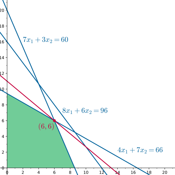
Next, we want to maximize \(z=5x_1+6x_2\). If we treat this equation as the line \(5x_1+6x_2=z\), then as \(z\) varies, we obtain a family of parallel lines, with larger \(z\) values corresponding to lines further to the upper right. Therefore, we only need to shift the line until it reaches a critical position where moving it slightly further to the upper right would cause it to no longer intersect the feasible region; the \(z\) value at this line is the desired maximum.

As shown in the figure, this occurs at the red point. It is the intersection of the lines \(4x_1 + 7x_2 = 66\) and \(7x_1 + 3x_2 = 60\). Solving the system of equations yields its coordinates as \((6,6)\). This is the unique optimal solution to the problem. The chef's maximum profit is \(z=66\).

When the problem involves more than two decision variables, the graphical method is no longer applicable. However, some observations from this example remain valid. Each inequality constraint in a linear programming problem describes a "half-space," and the set of all feasible solutions is the intersection of these "half-spaces," which is always a "convex polyhedron." The optimal solution of the programming problem can always be attained at some "vertex" of this "convex polyhedron." The coordinates of these "vertices" can be obtained by solving the equations of the "boundaries" of these "half-spaces." Extending these observations to higher dimensions leads to an efficient method for solving linear programming problems—the simplex method. This is also the most commonly applied method in algorithmic contests.

Another noteworthy point is that, in principle, the number of steamed buns and fried dough sticks produced by the chef should be integers, as they are not infinitely divisible. Although this integer restriction is not explicitly enforced in the solution process, since the final optimal solution happens to be integers, the answer remains feasible even with the integer constraint. However, for many programming problems, the optimal solution may not occur at integer points; such problems are actually integer programming problems rather than simple linear programming problems. The end of this article briefly discusses such problems.

Basic Concepts

This section introduces the basic concepts of linear programming problems.

Linear Programming Problem

A linear programming problem \(P\) typically consists of two parts:

• A linear objective function, i.e., a function of the form

  \[ f(x_1,x_2,\cdots,x_n)=c_1x_1+c_2x_2+\cdots+c_nx_n \]

  where \(c_i\in\mathbf R\) are constants;

• Linear constraints, i.e., inequality or equality constraints of the form

  \[ g_j(x_1,x_2,\cdots,x_n)=a_{j1}x_1+a_{j2}x_2+\cdots+a_{jn}x_n \le (=,\ge) b_j \]

  where \(a_{ji},b_j\in\mathbf R\) are constants.

A linear programming problem aims to maximize or minimize the objective function subject to the given constraints. A solution \((x_1,x_2,\cdots,x_n)\in\mathbf R^n\) satisfying the constraints is called a feasible solution; among all feasible solutions, the one that optimizes the objective function is called an optimal solution.

Standard Form

For convenience in description and further processing, it is common to specify a standard form for linear programming problems. Different literature may adopt different conventions; this article defines the standard form as follows:

\[ \begin{aligned} \min_{\{x_i\}}\;& \sum_{i=1}^n c_ix_i \\ \text{subject to }& \sum_{i=1}^n a_{ji}x_i = b_i \ge 0,~j=1,\cdots,m,\\ & x_i \ge 0,~i = 1,\cdots,n. \end{aligned} \]

That is, the linear programming problem is a minimization problem, all decision variables have non-negativity constraints, and aside from these, it only contains several equality constraints with non-negative right-hand side constants. Using matrices, this problem can be expressed more concisely:

\[ \max\{c^Tx : Ax = b \ge 0,~ x\ge 0\}. \]

Here, \(x=(x_i)\in\mathbf R^n\) are the decision variables, \(b=(b_j)\in\mathbf R^m\) and \(A=(a_{ji})\in\mathbf R^{m\times n}\) are constants involved in the constraints. The size of a linear programming problem refers to the number of its decision variables and the number of its constraints.

Vector Inequality

This article frequently uses vector inequalities like \(b \ge 0\). Generally, for vectors \(x,y\in\mathbf R^n\), the inequality \(x\le y\) means \(\forall i(x_i\le y_i)\), i.e., component-wise comparison in the real number sense. This relation is a partial order on the vector space, meaning there exist pairs of vectors that are incomparable.

The choice of standard form is merely for convenience and has no special significance, as any linear programming problem can be equivalently written in one of the following six forms:

\[ \begin{aligned} &\min\{c^Tx : Ax = b,~ x\ge 0\},\\ &\min\{c^Tx : Ax \ge b\},\\ &\min\{c^Tx : Ax \ge b,~ x\ge 0\},\\ &\max\{c^Tx : Ax = b,~ x\ge 0\}, \\ &\max\{c^Tx : Ax \le b\},\\ &\max\{c^Tx : Ax \le b,~ x\ge 0\}.\\ \end{aligned} \]

The following operations can equivalently transform any linear programming problem into one of these six forms:

1. By adding a negative sign, i.e., changing \(c\) to \(-c\), maximization and minimization problems can be interconverted.
2. By adding a negative sign, i.e., replacing \(a_j^Tx \lesseqqgtr b_j\) with \(-a_j^Tx \gtreqqless -b_j\), the two directions of inequality constraints can be interconverted, or the right-hand side constants of equality constraints can be made non-negative.
3. All equality constraints \(a_j^Tx = b_j\) can be replaced by two opposite inequality constraints \(a_j^Tx \ge b_j\) and \(a_j^Tx \le b_j\).
4. All inequality constraints \(a_j^Tx \le(\ge) b_j\) can be converted into equality constraints \(a_j^Tx +(-) s_j = b_j\) and corresponding non-negativity constraints \(s_j\ge 0\) by introducing non-negative slack variables \(s_j\).
5. If a decision variable \(x_i\) lacks a non-negativity constraint, it can be replaced by the difference of two non-negative variables, i.e., \(x_j = x^+_j - x^-_j\) with \(x^+_j,x^-_j \ge 0\).

The size of the linear programming problem obtained through these transformations is at most twice that of the original problem, and the feasible and optimal solutions of these problems are easily interconverted. Therefore, for a general linear programming problem, it is always possible to first convert it into standard form (or one of the six forms above) before solving.

Example

Consider the linear programming problem

\[ \begin{aligned} \max\;& 3x_1 - 2x_2 + x_3 \\ \text{subject to }& 2x_1 + 3x_2 + 4x_3 \ge 1,\\ & 3x_1 + 4x_2 \le 5,\\ & 5x_2 - x_3 = -1, \\ & x_1, x_2 \ge 0. \end{aligned} \]

Using operations 1, 2, and 3, it can be transformed into the form \(\min\{c^Tx : Ax \ge b\}\), i.e.,

\[ \begin{aligned} \min\;& -3x_1 + 2x_2 - x_3 \\ \text{subject to }& 2x_1 + 3x_2 + 4x_3 \ge 1,\\ & -3x_1 - 4x_2 \ge -5,\\ & 5x_2 - x_3 \ge -1, \\ & -5x_2 + x_3 \ge 1, \\ & x_1 \ge 0,\\ & x_2 \ge 0. \end{aligned} \]

Using operations 4 and 5, it can be transformed into the form \(\max\{c^Tx : Ax = b,~ x\ge 0\}\), i.e.,

\[ \begin{aligned} \max\;& 3x_1 - 2x_2 + x^+_3 - x^-_3 \\ \text{subject to }& 2x_1 + 3x_2 + 4x^+_3 - 4x^-_3 - x_4 = 1,\\ & 3x_1 + 4x_2 + x_5 = 5,\\ & 5x_2 - x^+_3 + x^-_3 = -1, \\ & x_1, x_2, x^+_3, x^-_3, x_4, x_5 \ge 0. \end{aligned} \]

Feasible Region and Solutions

The set of all feasible solutions \(\mathcal D\subseteq\mathbf R^n\) is called the feasible region of the linear programming problem \(P\). Geometrically, each inequality constraint \(a_j^T x \le b_j\) describes a half-space \(\{x\in\mathbf R^n:a_j^T x \le b_j\}\), and each equality constraint \(a^T_jx = b_j\) describes a hyperplane \(\{x\in\mathbf R^n:a_j^Tx=b_j\}\). Therefore, the feasible region is always the intersection of finitely many half-spaces and hyperplanes. In optimization literature¹, such geometric objects are usually called polyhedra in \(\mathbf R^n\). A polyhedron is always a closed convex set but not necessarily bounded. A bounded polyhedron is also called a polytope. A polytope can be seen as a generalization of polygons in the plane to higher dimensions, while polyhedra further generalize to possibly unbounded cases.

Examples of Polyhedra

Here are some common polyhedra:

1. The empty set \(\varnothing\), also called the nullitope, whose dimension is defined as \(-1\).
2. Affine subspaces, i.e., intersections of hyperplanes \(\{x\in\mathbf R^n:Ax = b\}\). This corresponds to the solution set of the linear system \(Ax = b\): if the system has no solution, it is empty; otherwise, it can always be written as \(x_0+V\), where \(x_0\in\mathbf R^n\) and \(V\subseteq\mathbf R^n\) is a linear subspace of dimension \(n-\operatorname{rank}(A)\). In particular, a hyperplane is also an affine subspace.
3. Polyhedral cones, i.e., the set of all non-negative linear combinations of finitely many points \(\{x_i\}\), \(\{\sum_i\alpha_ix_i:\alpha_i\ge 0\}\). It is a convex cone with its vertex at the origin. Equivalently, it can be viewed as a polyhedron bounded by several hyperplanes passing through the origin, i.e., \(\{x\in\mathbf R^n : Ax\le 0\}\). In particular, a half-space is also a polyhedral cone.
4. Polytopes, i.e., bounded polyhedra. In particular, polytopes of dimension \(-1\), \(0\), \(1\), \(2\), \(3\) are the common empty set, points, line segments, polygons, and (ordinary) polyhedra. A set is a polytope if and only if it is the convex hull of finitely many points \(\{x_i\}\), \(\{\sum_i\alpha_ix_i:\alpha_i\ge 0,~\sum_i\alpha_i=1\}\). A \(k\)-dimensional polytope is at least the convex hull of \(k+1\) points.
5. Simplices, i.e., \(k\)-dimensional polytopes generated by exactly \(k+1\) points. They are the simplest \(k\)-dimensional polytopes. In particular, polytopes of dimension \(-1\), \(0\), \(1\), \(2\), \(3\) are the empty set, points, line segments, triangles, and tetrahedra, respectively. The simplest example of a \(k\)-dimensional simplex is \(\{x\in\mathbf R^k:x_i\ge 0,~\sum_ix_i=1\}\). In fact, any \(k\)-dimensional simplex can be transformed into such a special case via affine transformations (i.e., translation and scaling). Notably, the simplex method does not actually operate on simplices.

Any polyhedron can be viewed as the Minkowski sum of a polyhedral cone and a polytope: the former describes the unbounded part of the polyhedron, while the latter describes the shape of the bounded part. This polyhedral cone is unique: the polyhedral cone obtained from decomposing the polyhedron \(\{x\in\mathbf R^n:Ax\le b\}\) is always \(\{x\in\mathcal R^n:Ax\le 0\}\).

The solutions of linear programming are closely related to the structure of polyhedra. For a polyhedron \(\mathcal D\in\mathbf R^n\) and a vector \(c\in\mathbf R^n\setminus\{0\}\), consider the following linear programming problem \(P\): (similar discussion applies to minimization)

\[ \max\{c^Tx:x\in\mathcal D\}. \]

Geometrically, this is equivalent to moving the hyperplane \(H:c^Tx = z\) along the direction of vector \(c\) to make \(z\) as large as possible, under the condition that \(H\) intersects the feasible region \(\mathcal{D}\). There are three possibilities:

• The feasible region \(\mathcal D\) is empty. This means problem \(P\) has no feasible solution; some of its constraints are contradictory. In this case, the problem \(P\) is called infeasible, and its optimal value is defined as \(-\infty\).

• The feasible region \(\mathcal D\) is non-empty but contains a ray with direction vector \(c\), i.e., there exists \(x_0\in\mathbf R^n\) such that \(x_0+tc\in\mathcal D\) for all \(t\ge 0\). Since the hyperplane \(H\) can be moved indefinitely along the direction of \(c\), and during this movement, the set \(H\cap\mathcal D\) always contains at least some point on this ray (hence non-empty), the objective function \(c^Tx = c^Tx_0 + tc^Tc\) can take arbitrarily large values. In this case, the problem \(P\) is called unbounded, and its optimal value is defined as \(+\infty\).

• The feasible region \(\mathcal D\) is non-empty and contains no ray with direction vector \(c\). In this case, the problem \(P\) is called bounded. Let \(z^*\in\mathbf R\) be the optimal value of problem \(P\). The hyperplane \(H^*:c^Tx = z^*\) is in a critical position: it intersects the polyhedron \(\mathcal D\), and \(\mathcal D\) is contained in the half-space \(\{x:c^Tx\le z^*\}\). Such a hyperplane is called a supporting hyperplane of the polyhedron \(\mathcal D\). The optimal solution set of problem \(P\) is \(H^*\cap\mathcal D\). As the intersection of a supporting hyperplane and a polyhedron, the set \(H^*\cap\mathcal D\) is always a polyhedron and lies on the boundary of \(\mathcal D\). It is called a face of the polyhedron \(\mathcal D\). Figuratively, a polyhedron is bounded by these faces. Besides these faces formed by intersections with supporting hyperplanes, a polyhedron generally has two additional faces: the empty set and the polyhedron itself. All faces of a polyhedron, under set inclusion, form a lattice structure.

  The dimension of a face of a \(d\)-dimensional polyhedron must be an integer between \(0\) and \(d\). Faces of dimension \(0\) (i.e., points) are called vertices or corner points of the polyhedron \(\mathcal D\); faces of dimension \(1\) are called edges; faces of dimension \(d-1\) are called facets. However, not all polyhedra have vertices. Since a face of a face is still a face of the polyhedron, and only affine subspaces have no strictly smaller non-empty faces, all minimal faces of a polyhedron are affine subspaces. Moreover, all minimal faces of the same polyhedron have the same dimension; in particular, the minimal faces of the polyhedron \(\mathcal D=\{x\in\mathbf R^n:Ax\le b\}\) have dimension \(n-\operatorname{rank}A\).

  Since the faces of a polyhedron are the solution sets of bounded linear programming problems, it is important to understand how to determine the equations of a polyhedron's faces. Suppose the polyhedron \(\mathcal D\) is described by several constraints \(a_j^Tx \lesseqqgtr b_j\), and \(F\) is a face of \(\mathcal D\). If a constraint holds with equality for all \(x\in F\), it is said to be tight on face \(F\). Points on face \(F\) obviously satisfy the system of equations obtained by setting these tight constraints to equality, and the intersection of the affine subspace determined by this system with the polyhedron \(\mathcal D\) is exactly face \(F\). Conversely, arbitrarily selecting a subset of the constraints of \(\mathcal D\), setting them to equality, solving the resulting system, and intersecting the affine subspace with \(\mathcal D\) yields a face of \(\mathcal D\). Moreover, the more tight constraints selected, the smaller the resulting face (in terms of inclusion).

  In particular, for the feasible region \(\mathcal D=\{x\in\mathbf R^n:Ax=b,~x\ge 0\}\) of a standard-form linear program, the coefficient matrix \(\begin{pmatrix}A\\ I\end{pmatrix}\) has rank \(n\), so its minimal faces are its vertices. That is, if the problem is bounded, its optimal solution can always be chosen as a vertex. Furthermore, this vertex can be obtained by selecting \(n\) linearly independent tight constraints and solving the system. This is the convenience of the standard form of linear programming.

Example

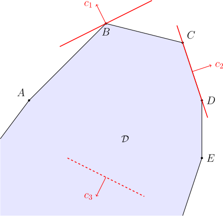
In the figure below, \(\mathcal D\) is the feasible region. When the coefficients in the objective function are \(c_1,c_2,c_3\), they correspond to the three cases of unique optimal solution, multiple optimal solutions, and unboundedness, respectively. For the first two cases, the corresponding thick red solid lines are (one of) the supporting hyperplanes of the solution set; the optimal solution sets are the vertex \(B\) and the edge \(\overline{CD}\) of the polyhedron \(\mathcal D\), respectively. For the third case, since the feasible region \(\mathcal D\) contains a ray with direction \(c_3\), the hyperplane with normal vector \(c_3\) can be moved continuously along \(c_3\), making the problem unbounded.

These discussions ignore the case \(c=0\). In that case, the linear programming problem obviously cannot be unbounded, so either the problem is infeasible, or the optimal value is \(0\), and the optimal solution set is \(\mathcal D\) itself. Such special linear programs are also called feasibility linear programming.

It is worth noting that determining whether a linear programming problem is feasible, bounded, or finding a feasible solution to a system of inequalities are problems as difficult as solving the linear programming problem itself². For example, the proof of the strong duality theorem below shows that solving a bounded linear programming problem is equivalent to finding a feasible solution to a system of inequalities. Therefore, the most effective way to determine whether a system of inequalities has a solution or whether a system of equations has a non-negative solution is to solve the corresponding feasibility linear program³.

Additionally, if a constraint of a linear programming problem is not tight on any face of the feasible region, then that constraint is redundant. In the breakfast chef example at the beginning of this article, the time constraint is a redundant constraint. Determining whether a given inequality \(a_j^Tx\le b_j\) in a system is redundant can be solved by solving the linear programming problem \(\max\{a_j^Tx:x\in\mathcal D\}\) and comparing it with \(b_j\).

Common Algorithms

In algorithmic contests, few problems can only be solved by linear programming algorithms. Most problems solvable by linear programming methods can usually also be solved by more specialized and efficient algorithms like network flow.

Common algorithms for solving linear programming problems include:

• Simplex method
• Ellipsoid method
• Interior-point method

Although the worst-case complexity of the simplex method is exponential, while interior-point methods have polynomial complexity, both types of algorithms perform exceptionally well in most practical problems. In contrast, although the ellipsoid method has polynomial theoretical complexity, it is usually slow and not practical.

It is still unknown whether linear programming problems admit strongly polynomial-time algorithms.

Duality

Every linear programming problem has a corresponding dual problem. The solutions of the primal and dual problems are closely related. Duality not only helps in deeper understanding of the problem structure but often also improves the efficiency of solving the primal problem.

For a linear programming problem \(P\) (all lowercase letters denote vectors)

\[ \begin{aligned} \min_{x_1,x_2,x_3}\;& c_1^Tx_1 + c_2^Tx_2 + c_3^Tx_3 \\ \text{subject to }& A_{11}x_1 + A_{12}x_2 + A_{13}x_3 \ge b_1,\\ & A_{21}x_1 + A_{22}x_2 + A_{23}x_3 = b_2,\\ & A_{31}x_1 + A_{32}x_2 + A_{33}x_3 \le b_3,\\ & x_1\ge 0,~ x_3\le 0, \end{aligned} \]

its dual problem \(D\) is the linear programming problem

\[ \begin{aligned} \max_{y_1,y_2,y_3}\;&b_1^Ty_1+b_2^Ty_2+b_3^Ty_3 \\ \text{subject to }&A_{11}^Ty_1 + A_{21}^Ty_2 + A_{31}^Ty_3\le c_1,\\ &A_{12}^Ty_1 + A_{22}^Ty_2 + A_{32}^Ty_3 = c_2,\\ &A_{13}^Ty_1 + A_{23}^Ty_2 + A_{33}^Ty_3 \ge c_3,\\ &y_1\ge 0,~ y_3\le 0. \end{aligned} \]

Here, the dual decision variables \(y_1,y_2,y_3\) are the Lagrange multipliers for the three types of constraints in the primal problem; conversely, the primal decision variables \(x_1,x_2,x_3\) are the Lagrange multipliers for the three types of constraints in the dual problem. It is easy to verify that the dual of the dual problem is the primal problem.

The correspondence between the primal problem \(P\) and the dual problem \(D\) is as follows:

Minimization Problem	Maximization Problem
Greater-than-or-equal constraint	Non-negative variable
Less-than-or-equal constraint	Non-positive variable
Equality constraint	Free variable
Non-negative variable	Less-than-or-equal constraint
Non-positive variable	Greater-than-or-equal constraint
Free variable	Equality constraint
Objective function coefficients	Constraint right-hand side constants
Constraint right-hand side constants	Objective function coefficients

In particular, the dual of the standard-form linear programming problem

\[ \min\{c^Tx:Ax=b,~x\ge 0\} \]

is

\[ \max\{b^Ty:A^Ty\le c\}. \]

Duality Principles

The primal and dual problems are not only mirror images in form but also closely related in their solutions. This is called the duality principle. For convenience, this section will use the standard-form primal problem in stating and proving theorems.

First, the weak duality theorem states that the maximum of the dual problem does not exceed the minimum of the primal problem.

Weak Duality Theorem

For all \(A\in\mathbf R^{m\times n}\), \(b\in\mathbf R^m\), and \(c\in\mathbf R^n\), we always have

\[ \max\{b^Ty:A^Ty\le c\} \le \min\{c^Tx:Ax=b,~x\ge 0\}. \]

Proof

If either the primal or dual problem is infeasible, the inequality holds trivially. Assume both problems are feasible. Then, for all feasible \(x\) and \(y\), we have

\[ b^Ty = x^TA^Ty \le x^Tc. \]

Therefore, taking the extremal values on both sides yields the weak duality theorem.

Based on the weak duality theorem, the solution status of the primal and dual problems can only be one of the following four cases:

1. Both primal and dual problems are infeasible, i.e., \(-\infty\le+\infty\);
2. Primal problem infeasible, dual problem unbounded, i.e., \(+\infty\le+\infty\);
3. Primal problem unbounded, dual problem infeasible, i.e., \(-\infty\le-\infty\);
4. Both primal and dual problems are bounded.

The weak duality theorem has many corollaries. For example, it actually provides a method to determine that a primal problem is unbounded using the feasibility of the dual problem.

Corollary

A linear programming problem is unbounded if and only if it is feasible and its dual problem is infeasible.

Applying the weak duality theorem to feasibility linear programming yields Farkas' lemma (and its variants).

Farkas' Lemma

For \(A\in\mathbf R^{m\times n}\) and \(b\in\mathbf R^n\), exactly one of the following holds:

1. There exists \(x\in\mathbf R^n\) such that \(Ax=b\) and \(x\ge 0\);
2. There exists \(y\in\mathbf R^m\) such that \(A^T y\ge 0\) and \(b^Ty<0\).

Proof

Consider the linear programming problem \(\max\{0:Ax=b,~x\ge 0\}\); its dual is \(\min\{b^Ty:A^Ty\ge 0\}\). The dual problem is obviously feasible because at least \(0\in\mathbf R^m\) is a feasible solution. Therefore, by the weak duality theorem, either the primal problem is feasible or the dual problem is unbounded, and these are mutually exclusive. Primal feasibility corresponds to case 1 in Farkas' lemma, and dual unboundedness is equivalent to case 2 in Farkas' lemma. This proves Farkas' lemma.

Farkas' lemma is actually a form of the hyperplane separation theorem. Case 1 says that point \(b\) lies within the polyhedral cone \(C\) generated by the column vectors of \(A\); therefore, Farkas' lemma states that if and only if point \(b\) is not in this convex cone \(C\), there exists a hyperplane \(H:y^Tx = 0\) passing through the origin with normal vector \(y\) that strongly separates point \(b\) and the polyhedral cone \(C\).

In fact, for the fourth case allowed by the weak duality theorem, a stronger conclusion holds: the optimal values of the primal and dual problems are equal. Combining the latter three cases gives the strong duality theorem: as long as either the primal or dual problem is feasible, their optimal values must be equal.

Strong Duality Theorem

For all \(A\in\mathbf R^{m\times n}\), \(b\in\mathbf R^m\), and \(c\in\mathbf R^n\), we have

\[ \max\{b^Ty:A^Ty\le c\} = \min\{c^Tx:Ax=b,~x\ge 0\}. \]

provided at least one of the two sets is non-empty.

Proof

The only case not covered by the weak duality theorem is when both primal and dual problems are feasible. In this case, consider the following feasibility linear programming problem \(Q\):

\[ \max\{0:c^Tx \le b^Ty,~Ax=b,~x\ge 0,~A^Ty\le c\}. \]

If problem \(Q\) has a feasible solution \((x^*,y^*)\in\mathbf R^n\times\mathbf R^m\), then by the weak duality theorem and optimality, we have

\[ b^Ty^* \le \max\{b^Ty:A^Ty\le c\} \le \min\{c^Tx:Ax=b,~x\ge 0\} \le c^Tx^*, \]

but \(c^Tx^*\le b^Ty^*\), so all these inequalities must hold with equality. That is, not only does strong duality hold, but \(x^*\) and \(y^*\) are optimal solutions for the primal and dual problems, respectively.

Therefore, we only need to prove that problem \(Q\) is feasible. Suppose not. Mimicking the proof of Farkas' lemma, consider the dual problem \(DQ\) of problem \(Q\):

\[ \min\{c^T\mu - b^T\lambda : ct - A^T\lambda \ge 0,~ -bt + A\mu = 0,~t\ge 0,~\mu\ge 0\}. \]

Since \((t,\lambda,\mu)=(0,0,0)\) is a feasible solution to the dual problem \(DQ\), by the weak duality theorem, the infeasibility of problem \(Q\) implies that the dual problem \(DQ\) is unbounded, i.e., there exists \((t^*,\lambda^*,\mu^*)\) such that

\[ c^T\mu^* - b^T\lambda^* <0,~ ct^* - A^T\lambda^* \ge 0,~ -bt^* + A\mu^* = 0,~t^*\ge 0,~\mu^*\ge 0. \]

Now, if \(t^*>0\), then these inequalities actually indicate that \((x,y)=(\mu^*/t^*,\lambda^*/t^*)\) is a feasible solution to the aforementioned problem, contradicting the assumption. Therefore, we must have \(t^*=0\). This implies

\[ c^T\mu^* < b^T\lambda^*,~ A^T\lambda^*\le 0,~ A\mu^*=0,~\mu^*\ge 0. \]

However, since we have assumed that the primal and dual problems in the theorem are both feasible, i.e., there exists \((x_0,y_0)\) such that

\[ Ax_0 = b,~ x_0\ge 0,~ A^Ty_0\le c \]

holds, we have

\[ 0 = (A\mu^*)^Ty_0 = (A^Ty_0)^T\mu^* \le c^T\mu^* < b^T\lambda^* = x_0^TA^T\lambda^* \le 0. \]

This is clearly a contradiction. This contradiction shows that problem \(Q\) is feasible, and hence strong duality holds.

From the proof of the strong duality theorem, we also obtain the following corollary:

Corollary

Let \(x^*\) and \(y^*\) be feasible solutions to the primal and dual problems, respectively, satisfying strong duality, i.e., \(c^Tx^* = b^Ty^*\). Then, they are also optimal solutions to the primal and dual problems, respectively.

The strong duality theorem shows that for a feasible linear programming problem, solving its dual problem yields the optimal value of the primal problem.

Complementary Slackness Conditions

Like other optimization problems, complementary slackness conditions are part of the optimality conditions for linear programming problems. Moreover, because the objective function is linear, for linear programming problems, complementary slackness conditions are both necessary and sufficient for a feasible solution to be optimal.

The complementary slackness condition states that a variable in the dual (primal) problem can take a non-zero value only if the corresponding constraint in the primal (dual) problem is tight (i.e., holds with equality). If treating a variable taking a non-zero value as a slack constraint, this means that corresponding variables and constraints in the primal and dual problems cannot both be slack simultaneously. Hence, this condition is called complementary slackness.

For standard-form linear programming problems, the following holds:

Theorem

Suppose \(x^*\) and \(y^*\) are feasible solutions to the primal problem \(\min\{c^Tx:Ax=b,~x\ge 0\}\) and the dual problem \(\max\{b^Ty:A^Ty\le c\}\), respectively. Then, \(x^*\) and \(y^*\) are optimal solutions to the primal and dual problems, respectively, if and only if the complementary slackness condition holds, i.e.,

\[ x^T(A^Ty-c) = 0. \]

Proof

Since \(x^*\) and \(y^*\) are feasible, we have

\[ b^Ty^* - c^Tx^* = (x^*)^T(A^T y^* - c). \]

Therefore, complementary slackness holds if and only if \(b^Ty^* = c^Tx^*\). By the corollary to the strong duality theorem, this condition holds if and only if \(x^*\) and \(y^*\) are optimal solutions.

The standard form might be too special. A slightly more general form of the theorem is as follows:

Theorem

Suppose \(x^*\) and \(y^*\) are feasible solutions to the primal problem \(\min\{c^Tx:Ax\ge b,~x\ge 0\}\) and the dual problem \(\max\{b^Ty:A^Ty\le c,~y\ge 0\}\), respectively. Then, \(x^*\) and \(y^*\) are optimal solutions to the primal and dual problems, respectively, if and only if the complementary slackness condition holds, i.e.,

\[ x^T(A^Ty-c) = y^T(Ax-b) = 0. \]

Proof

The proof is essentially the same, but this time we write the difference as

\[ b^Ty^* - c^Tx^* = (x^*)^T(A^T y^* - c) - (y^*)^T(Ax^*-b). \]

Complementary slackness conditions provide a simple criterion for checking the optimality of feasible solutions to linear programming problems.

Primal-Dual Method

The dual problem can assist in solving the primal problem. A commonly used method in solving linear programming problems is the primal-dual method. It solves a series of relatively simple auxiliary problems, gradually improving the dual solution, and eventually obtaining the optimal solution to the primal problem.

For the standard-form primal problem

\[ (P)\qquad\min\{c^Tx : Ax=b\ge 0,~ x\ge 0\} \]

and its dual problem

\[ (D)\qquad\max\{b^Ty : A^Ty\le c\}, \]

the previous section showed that to find their optimal solutions, we only need to find a pair of feasible solutions to \((P)\) and \((D)\) that satisfy the complementary slackness condition \(x^T(A^Ty-c)=0\). Consider the following procedure:

1. Start from a feasible solution \(y\) to the dual problem \((D)\), and compute the set of tight constraints for the dual problem:

   \[ I = \{i : (A^Ty - c)_i = 0\}. \]

2. According to complementary slackness, if there exists a feasible solution \(x\) to problem \((P)\) such that \(x_i>0\) only for \(i\in I\), then we have found an optimal pair. Therefore, consider the linear programming problem

   \[ (RP)\qquad \begin{aligned} \min_{x,s}\;& \mathbf 1^Ts \\ \text{subject to } & Ax + s = b, \\ & x_i \ge 0,~\forall i \in I,\\ & x_i = 0,~\forall i \notin I,\\ & s \ge 0. \end{aligned} \]

3. If the minimum value of problem \((RP)\) is \(0\), then the \(x^*\) in the optimal solution \((x^*,0)\) is an optimal solution to the primal problem \((P)\). Otherwise, we can find the solution \(\bar y\) to its dual problem \((DRP)\):

   \[ (DRP)\qquad \begin{aligned} \max_{y}\;& b^Ty \\ \text{subject to }& \sum_{j}a_{ji}y_j \le 0,~\forall i\in I,\\ & y \le 1. \end{aligned} \]

   By the strong duality theorem, \(b^T\bar y = 1^Ts^*>0\).

4. Improve the feasible solution to the dual problem \((D)\) using the solution from \((DRP)\). Let \(y' = y + \varepsilon \bar y\), where \(\varepsilon>0\). Then \(b^Ty' = b^Ty + \varepsilon b^T\bar y > b^Ty\). Therefore, to ensure \(y'\) remains feasible for \((D)\), we choose \(\varepsilon\) as large as possible.

   For \(i\in I\), we have

   \[ \sum_ja_{ji}y'_j = \sum_ja_{ji}y_j + \varepsilon \sum_ja_{ji}\bar y_j \le c_i, \]

   so these constraints of problem \((D)\) are always satisfied.

   For the remaining constraints, i.e., for \(i\notin I\), we take

   \[ \varepsilon = \min\left\{\dfrac{c_i - \sum_{j}a_{ji}y_j}{\sum_{j}a_{ji}\bar y_j}:i\notin I,~\textstyle\sum_{j}a_{ji}\bar y_j>0\right\} \]

   to improve the dual solution as much as possible while maintaining feasibility, then return to step 1 and continue iterating. In particular, if the set in the above expression is empty, i.e., \(\varepsilon=+\infty\), then the dual problem \((D)\) is unbounded, and the primal problem \((P)\) is infeasible.

In this process, only problem \((DRP)\) actually needs to be solved; it is linked to problem \((RP)\) via the strong duality theorem. Problem \((DRP)\) provides a direction to improve the dual solution, and compared to the dual problem \((D)\) itself, problem \((DRP)\) has a simpler form. The feasibility of problem \((DRP)\) is guaranteed by Farkas' lemma, and the constraint \(y\le 1\) is just a normalization condition ensuring \((DRP)\) is bounded.

In algorithmic contests, the primal-dual method is widely applied to various combinatorial optimization problems. For example, the Hungarian algorithm for maximum weight bipartite matching, the cycle cancellation algorithm and SSP algorithm (primal-dual algorithm) for minimum cost flow, Dijkstra's algorithm for shortest paths, and the Ford–Fulkerson augmenting path algorithm for maximum flow can all be viewed as direct applications of the primal-dual method.

Integer Programming

Integer programming usually refers to integer linear programming (ILP). The standard form of integer linear programming is:

\[ \begin{aligned} \min_{x}\; & c^Tx \\ \text{subject to } & Ax = b \ge 0,\\ & x \ge 0,\\ & x \in \mathbf Z^n, \end{aligned} \]

where \(A\in\mathbf R^{m\times n}\), \(b\in\mathbf R^m\), \(c\in\mathbf R^n\). That is, integer linear programming is obtained by adding the constraint that decision variables must be integers to a linear programming problem.

The integer constraint significantly increases the complexity of integer programming problems. Many combinatorial optimization problems, such as the knapsack problem, satisfiability problems, and numerous graph-theoretic optimization problems, can be formulated as integer programming models, and most of these problems are proven to be NP-hard.

Totally Unimodular Matrices

Because of this, for many large-scale integer optimization problems, one sometimes considers relaxing the integer constraints and solving a linear programming problem instead. Generally, the optimal value of the relaxed linear programming problem is only a lower bound estimate for the original integer programming problem (assuming minimization). However, if the optimal solution of the relaxed linear programming problem happens to be integer, then it is also an optimal solution to the original integer programming problem.

A natural question is: are there conditions that guarantee the optimal solution of a linear programming problem is integer? The concept of totally unimodular matrices provides such a condition.

Totally Unimodular Matrix

A matrix \(A\in\mathbf R^{m\times n}\) is called totally unimodular if all its square submatrices have determinant \(0\) or \(\pm 1\).

In particular, all entries of a totally unimodular matrix are \(0\) or \(\pm 1\). Using this concept, we can state the following result:

Theorem

For a totally unimodular matrix \(A\in\mathbf Z^{m\times n}\), \(b\in\mathbf Z^{m}\), and \(c\in\mathbf Z^n\), the linear programming problem and its dual

\[ \min\{c^Tx : Ax=b,x\ge 0\} = \max\{b^Ty: A^Ty\le c\} \]

both have integer optimal solutions, provided they are bounded.

Proof

As mentioned earlier, the optimal solution set of a linear programming problem can be taken as one of its minimal faces, which is the solution set of a system of equations obtained by setting a set of linearly independent tight constraints to equality:

\[ \{x\in\mathbf R^n : a_j^Tx = b_j,~\forall j\in J\}. \]

Denote this system as \(A_Jx=b_J\), and write \(A_J=(A_1,A_2)\), where \(A_1\) is a full-rank square matrix with determinant \(\pm 1\). Then, by Cramer's rule, the solution

\[ x = \begin{pmatrix}A_1^{-1}b_J \\ 0\end{pmatrix} \]

is an integer solution on the minimal face.

In common graph-theoretic models, the coefficient matrices of linear programming problems corresponding to network flow, shortest paths, bipartite graphs, etc., are all totally unimodular. Therefore, as long as these problems involve only integer parameters, their optimal solutions can be taken as integers without worrying about fractional flows, fractional matchings, etc. Thus, problems like maximum flow, minimum cut, minimum cost flow, shortest path, difference constraints, maximum (weight) matching and minimum vertex cover in bipartite graphs can all be solved by transforming them into linear programming problems. Moreover, maximum flow and minimum cut, shortest paths and difference constraints, maximum bipartite matching and minimum vertex cover are pairwise dual problems.

Besides these, there are other common graph-theoretic models where all feasible solutions happen to be the vertices of a polytope with integer vertices. Therefore, by cleverly selecting constraints, the solutions of the corresponding combinatorial optimization problem coincide with the optimal solutions of some linear programming problem. For example, general graph matching and spanning tree models fall into this category, so problems like maximum (weight) matching in general graphs and minimum spanning tree can also be transformed into linear programming problems.

References and Notes

• Schrijver, Alexander. Theory of linear and integer programming. John Wiley & Sons, 1998.
• Papadimitriou, Christos H., and Kenneth Steiglitz. Combinatorial optimization: algorithms and complexity. Courier Corporation, 1998.
• Duality in linear programming. Part 1—definition and construction. by adamant - Codeforces blog
• Duality in linear programming. Part 2—in competitive programming. by adamant - Codeforces blog

---

1. Different literature may have different definitions for these terms: some refer to the bounded case as "polyhedron" and the unbounded case as "polytope"; some do not assume they are necessarily convex; some use "polyhedron" to refer to three-dimensional polytopes. This article adopts definitions consistent with Schrijver (1998) and Boyd and Vandenberghe (2004). ↩

2. More precisely, they are polynomial-time reducible to each other. ↩

3. Other methods for solving systems of inequalities include Fourier–Motzkin elimination and the Agmon–Motzkin–Schoenberg relaxation method. They are more direct but often inefficient. ↩

---

本页面最近更新：，更新历史
发现错误？想一起完善？ 在 GitHub 上编辑此页！
本页面贡献者：OI-wiki
本页面的全部内容在 CC BY-SA 4.0 和 SATA 协议之条款下提供，附加条款亦可能应用