Closest Pair of Points
Introduction
Given \(n\) points on a two-dimensional plane, find a pair of points with the smallest Euclidean distance.
Below we introduce a divide-and-conquer algorithm with time complexity \(O(n\log n)\) to solve this problem. This algorithm was proposed in 1975 by Franco P. Preparata. Preparata and Michael Ian Shamos proved that this algorithm is optimal under the decision tree model.
Process
As with conventional divide-and-conquer algorithms, we split the set of \(n\) points into two equally sized subsets \(S_1\) and \(S_2\), and recursively proceed. However, we encounter a challenge: how to merge? That is, how to find the closest pair where one point lies in \(S_1\) and the other in \(S_2\)? Here we first assume that the merge operation takes \(O(n)\) time, so the overall complexity of the algorithm is \(T(n) = 2T(\frac{n}{2}) + O(n) = O(n\log n)\).
We first sort all points by \(x_i\) as the primary key and \(y_i\) as the secondary key. Then, using point \(p_m (m = \lfloor \frac{n}{2} \rfloor)\) as the dividing point, we split the point set into \(A_1\) and \(A_2\):
We recursively compute the closest pair within each subset, obtaining distances \(h_1\) and \(h_2\), and set \(h = \min(h_1, h_2)\).
Now it's time to merge! We attempt to find a pair of points, one from \(A_1\) and the other from \(A_2\), with distance less than \(h\). Therefore, we collect all points whose horizontal distance from \(x_m\) is less than \(h\) into set \(B\):
Combined with the image, line \(m\) divides the points into two parts. The left side of \(m\) is point set \(A_1\), and the right side is point set \(A_2\).
According to the rule \(B = \{ p_i \ \big | \ \lvert x_i - x_m \rvert < h \}\), we obtain the green points forming set \(B\). 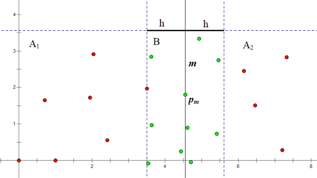
For each point \(p_i\) in \(B\), our current goal is to find another point also in \(B\) whose distance to \(p_i\) is less than \(h\). To avoid mutual consideration between two points, we only consider points with a \(y\)-coordinate less than \(y_i\). Clearly, for a valid point \(p_j\), we must have \(y_i - y_j < h\). Thus we obtain a set \(C(p_i)\):
Selecting a point \(p_i\) from set \(B\), according to the rule \(C(p_i) = \{ p_j\ \big |\ p_j \in B,\ y_i - h < y_j \le y_i \}\), we obtain set \(C\) consisting of the yellow points within the red box.
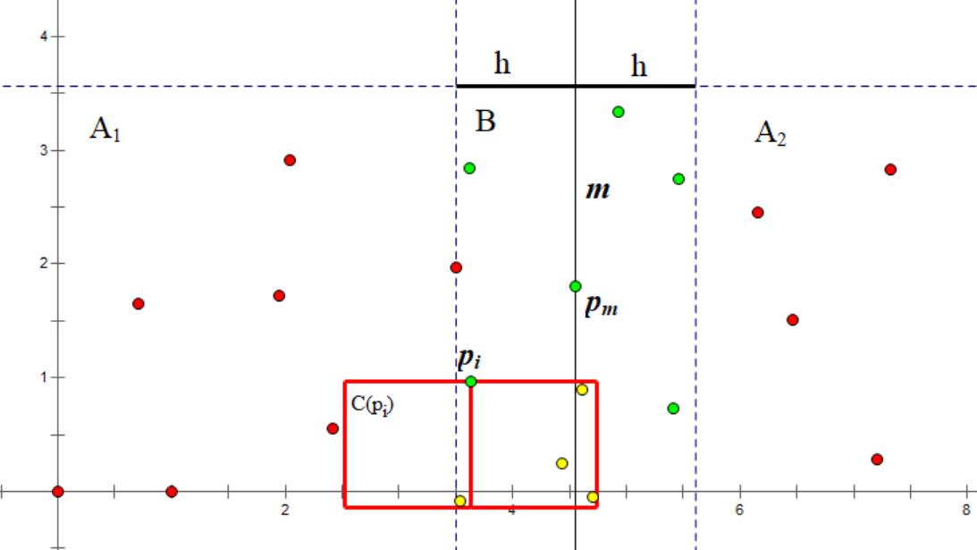
If we sort the points in \(B\) by \(y_i\), \(C(p_i)\) can be easily obtained as the few consecutive points immediately preceding \(p_i\).
Thus we derive the merging steps:
- Construct set \(B\).
- Sort the points in \(B\) by \(y_i\). The usual approach takes \(O(n\log n)\), but we can change strategy to optimize it to \(O(n)\) (explained below).
- For each \(p_i \in B\), consider \(p_j \in C(p_i)\). For each pair \((p_i,p_j)\), compute the distance and update the answer (the closest pair in the current set).
Note that we mentioned sorting twice above. Since point coordinates remain unchanged throughout, the first sort can be performed only once before the divide-and-conquer begins. We let each recursive call return the current point set sorted by \(y_i\). For the second sort, the upper level can directly merge the two already sorted point sets from the lower level.
It might seem that this algorithm is still not optimal, as \(|C(p_i)|\) could be on the order of \(O(n)\), leading to incorrect total complexity. However, this is not the case; its maximum size is \(7\), and we provide a proof:
Complexity Proof
We already know that all points in \(C(p_i)\) have \(y\)-coordinates in the range \((y_i-h, y_i]\); and all points in \(C(p_i)\), including \(p_i\) itself, have \(x\)-coordinates in the range \((x_m-h, x_m+h)\). This forms a \(2h \times h\) rectangle.
We further split this rectangle into two \(h \times h\) squares. Ignoring \(p_i\), the points in one square belong to \(C(p_i) \cap A_1\), and those in the other belong to \(C(p_i) \cap A_2\). Moreover, the distance between any two points within the same square is greater than \(h\) (because they come from the same lower-level recursion).
We divide a \(h \times h\) square into four \(\frac{h}{2} \times \frac{h}{2}\) small squares. It can be observed that each small square contains at most \(1\) point: because the maximum distance between any two points in such a small square is the length of its diagonal, i.e., \(\frac{h}{\sqrt 2}\), which is less than \(h\).
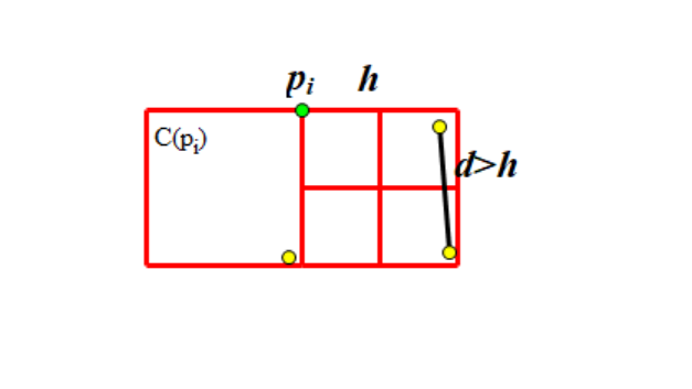
Thus, each square contains at most \(4\) points, the rectangle contains at most \(8\) points, and excluding \(p_i\) itself, \(\max(C(p_i))=7\).
Reference Implementation
1 2 3 4 5 6 7 8 9 10 11 12 13 14 15 16 17 18 19 20 21 22 23 24 25 26 27 28 29 30 31 32 33 34 35 36 37 38 39 40 41 42 43 44 45 46 47 48 49 50 51 52 53 54 55 56 57 58 59 60 61 62 63 64 65 66 67 68 69 70 | |
Extension: Minimum Perimeter Triangle in the Plane
The above algorithm interestingly extends to this problem: among a given set of points, choose three points such that the sum of their pairwise distances is minimized.
The algorithm remains largely unchanged. Each time we attempt to find a triangle with perimeter smaller than the current answer \(d\), we collect all points whose horizontal distance from \(x_m\) is less than \(\frac{d}{2}\) into set \(B\), and try to update the answer. (The longest side of a triangle with perimeter \(d\) is less than \(\frac{d}{2}\).)
Non-Divide-and-Conquer Algorithm
In fact, besides the divide-and-conquer algorithm mentioned above, there is another non-divide-and-conquer algorithm with time complexity also \(O(n \log n)\).
We can consider a common idea for statistical sequences: for each element, add its contribution with all elements to its left into the answer. The planar closest pair problem can also use this idea.
Specifically, we sort all points by \(x_i\) as the primary key and \(y_i\) as the secondary key, and maintain a multiset keyed by \(y_i\). For each position \(i\), we perform the following operations:
- Remove all points satisfying \(x_i - x_j \ge d\) from the set. They will no longer contribute to the answer.
- For all points in the set satisfying \(\lvert y_i - y_j \rvert < d\), compute their distance to \(p_i\).
- Insert \(p_i\) into the set.
Since each point is inserted and deleted at most once, the time complexity for insertion and deletion is \(O(n \log n)\). The proof for the time complexity of the answer computation part is similar to that of the divide-and-conquer algorithm, which the reader may attempt.
Reference Implementation
1 2 3 4 5 6 7 8 9 10 11 12 13 14 15 16 17 18 19 20 21 22 23 24 25 26 27 28 29 30 31 32 33 34 35 36 37 38 39 40 41 42 43 44 45 46 47 48 49 50 51 52 53 54 55 56 57 58 59 60 61 62 | |
Expected Linear Approach
Actually, besides the \(O(n \log n)\) approach mentioned above, there is also an algorithm with expected complexity \(O(n)\).
First, randomly shuffle the point pairs (random shuffle). We will maintain the answer for the prefix point sets. Consider computing the answer for the \(i\)-th point from the first \(i - 1\) points.
Let the closest pair distance among the first \(i - 1\) points be \(s\). We partition the plane into grids with side length \(s\), store the points in each grid (using a hash table), and then check all points in the nine grids surrounding the grid containing the \(i\)-th point, updating the answer. Note that the number of points to check is \(O(1)\), because the closest pair distance among the first \(i - 1\) points is \(s\), so each grid contains at most \(4\) points.
If during this process the answer is updated, we reconstruct the grid map; otherwise, we do not. Among the first \(i\) points, the probability that the closest pair includes \(i\) is \(O\left(\frac{1}{i}\right)\), and the cost of reconstructing the grid is \(O(i)\), so the expected cost for the \(i\)-th point is \(O(1)\). Thus, for \(n\) points, the expected complexity of this algorithm is \(O(n)\).
Exercises
- UVa 10245 "The Closest Pair Problem"[Difficulty: Low]
- SPOJ #8725 CLOPPAIR "Closest Point Pair"[Difficulty: Low]
- CODEFORCES Team Olympiad Saratov - 2011 "Minimum amount"[Difficulty: Medium]
- SPOJ #7029 CLOSEST "Closest Triple"[Difficulty: Medium]
- Google Code Jam 2009 Final "Min Perimeter"[Difficulty: Medium]
References and Further Reading
The divide-and-conquer algorithm part of this page is mainly translated from the blog post Нахождение пары ближайших точек and its English translation Finding the nearest pair of points. The Russian version's license is Public Domain + Leave a Link; the English version's license is CC-BY-SA 4.0.
Zhihu Column: Computational Geometry - Closest Pair Problem
本页面最近更新:,更新历史
发现错误?想一起完善? 在 GitHub 上编辑此页!
本页面贡献者:OI-wiki
本页面的全部内容在 CC BY-SA 4.0 和 SATA 协议之条款下提供,附加条款亦可能应用