2D Computational Geometry Basics
We restrict the geometric problems to be solved within the two-dimensional plane, which involves basic knowledge of 2D computational geometry. When studying, it is common to place figures in a Cartesian coordinate system or polar coordinate system, making problem-solving much more convenient.
Prerequisites
If you are not familiar with:
- Geometric fundamentals
- Cartesian coordinate system
- Vectors (including cross product)
- Polar coordinates and polar coordinate system
Please read Vectors and Polar Coordinates first.
Representing Geometric Figures
Points
In the Cartesian coordinate system, a point is represented by its x and y coordinates, such as point \((5,2)\), point \((-1,0)\), etc. Since coordinates are ordered pairs, they can be stored using std::pair or by defining a struct.
In the polar coordinate system, a point is represented by its radial distance and polar angle, and can be stored similarly to Cartesian coordinates.
Vectors
Since vectors are represented by coordinates in the same way as points, they can be stored just like points.
In the polar coordinate system, the same principle applies.
Lines
Representing lines in polar coordinates is relatively difficult, so we only discuss the Cartesian coordinate system.
Lines and Rays
In mathematical problems, lines are usually represented by equations. Common forms include the general form \(Ax+By+C=0\), slope-intercept form \(y=kx+b\), and intercept form \(\dfrac{x}{a}+\dfrac{y}{b}=1\). However, these forms are primarily used for analytical solutions. In computational geometry, using equations can increase the difficulty of solving problems.
In computational geometry, a line is typically represented by a point on the line and a direction vector. A ray is represented by its endpoint and a direction vector. A direction vector is a nonzero vector parallel to the line, usually taken as a unit vector. For a line, there are two unit vectors parallel to it; either can be chosen depending on the problem. For a ray, the direction vector is usually the one pointing in the direction the ray extends.
Line Segments
A line segment can be represented simply by its two endpoints.
Polygons
An array is used to record the vertices of the polygon in a specific order. For simple polygons, vertices are usually recorded in clockwise or counterclockwise order.
Specifically, for rectangles whose sides are parallel to the coordinate axes, it suffices to record the two diagonal vertices.
Curved Figures
Special curves, such as function graphs, are usually represented by their equations. For circles, simply record the center and radius.
Basic Formulas
Law of Sines
In \(\triangle \text{ABC}\), if angles \(A,B,C\) correspond to sides \(a,b,c\) respectively, then:
where \(R\) is the circumradius of \(\triangle \text{ABC}\).
Law of Cosines
In \(\triangle \text{ABC}\), if angles \(A,B,C\) correspond to sides \(a,b,c\) respectively, then:
The proofs of the above formulas are omitted. They are covered in the Chinese high school mathematics curriculum (人教版高中数学 A 版必修二, old edition: 必修五).
Basic Operations
Determining Which Side of a Line a Point Lies On
Given a point \(P\) on a line and the line's direction vector \(\mathbf v\), we want to determine which side of the line a point \(Q\) lies on. The "side" here is relative to the direction vector, meaning we face the direction pointed by the direction vector when making the judgment.
We use the properties of the cross product to compute \(\mathbf v\times \overrightarrow {PQ}\). According to the right-hand rule, if the cross product is negative, \(Q\) is on the right side of the line; if it is \(0\), \(Q\) is on the line; if it is positive, \(Q\) is on the left side of the line.
Quick Rejection Test and Straddle Test
We now want to determine whether two line segments intersect.
First, handle special cases. If the two segments are parallel, they obviously cannot intersect. This can be checked by comparing the slopes of the lines containing the segments.
Of course, if the segments overlap partially or entirely, or if the intersection point is an endpoint of one segment, we only need to check for collinearity of three points.
There are also obviously non-intersecting cases, colloquially described as "the two segments are too far apart." Define the "region of a segment" as the rectangle with sides parallel to the coordinate axes and the segment as its diagonal. Then, if two segments have no overlapping region, they definitely do not intersect.
For example, consider the following two segments:
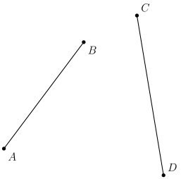
Their occupied regions are:
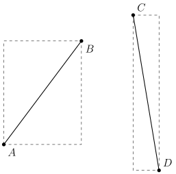
Thus, we can quickly determine that these two segments do not intersect.
This is the Quick Rejection Test. The above situation is called failing the quick rejection test.
Failing the quick rejection test is a sufficient but not necessary condition for two segments having no intersection; further judgment is needed.
If two segments \(a\) and \(b\) intersect, the two endpoints of segment \(b\) must lie on opposite sides of the line containing segment \(a\); similarly, the two endpoints of segment \(a\) must lie on opposite sides of the line containing segment \(b\). We can directly check the positions of the endpoints of one segment relative to the line containing the other segment. If they differ, the segments intersect; otherwise, they do not. As mentioned in the previous section, the position relationship between a line and a point can be determined using the cross product.
This is the Straddle Test. For two segments \(a\) and \(b\), if the two endpoints of \(b\) lie on opposite sides of the line containing \(a\), and the two endpoints of \(a\) lie on opposite sides of the line containing \(b\), we say \(a\) and \(b\) pass the straddle test, i.e., they intersect.
Note that two collinear but non-intersecting segments can also pass the straddle test. Therefore, accurate judgment requires combining it with the quick rejection test.
Determining Whether a Point Is Inside a Polygon
In computational geometry, this is known as the PIP problem. Several mature solutions exist, described below.
Ray Casting Algorithm
The original idea can be seen here.
First, handle special cases, such as "the point is too far from the polygon." Similar to judging segment intersection, consider the minimal axis-aligned bounding rectangle covering the polygon. If the point is not within this rectangle, it is definitely outside the polygon. This rectangle is easy to compute: take the minimum and maximum x and y coordinates of the polygon vertices, and combine them to form the four corners.
Also, if the point lies on an edge or vertex of the polygon, it is easy to check. For each edge, check if the point lies on the edge or at a vertex.
Consider drawing a ray starting from the point. If this ray intersects the polygon an odd number of times, the point is inside the polygon; otherwise, it is outside. We abbreviate this as odd in, even out. This algorithm is also known as the Even-odd rule.
Due to the Jordan curve theorem, each time the ray crosses a polygon edge, it toggles the inside/outside relationship. Thus, counting the parity of intersections suffices.
For the ray, you can randomly choose its slope; it is recommended to use an irrational number to avoid the ray coinciding with an edge.
In the original code, the last point in the polygon array is used as a point on the ray. When counting, if the ray passes through an edge or vertex, we can define that the point lies on one side of the ray and apply the straddle test.
Note
The ray casting algorithm only works for simple polygons. It does not apply to self-intersecting polygons because the Jordan curve theorem does not hold, making judgment impossible.
Winding Number Algorithm
The winding number is a mathematical concept representing the total number of times a closed curve winds counterclockwise around a point. It is easy to see that when the winding number is \(0\), the point is outside the curve. This algorithm is also known as the Nonzero-rule.
How to compute it? Connect the point to all vertices of the polygon and sum the signed angles between adjacent edges. Note that the angles are directed. If the sum is \(0\), the point is outside the polygon; otherwise, it is inside.
Finding the Intersection of Two Lines
First, determine if the two lines intersect by checking if their direction vectors are parallel. If the direction vectors are parallel, the lines are parallel, and the number of intersections is \(0\). Further, if the lines are parallel and pass through the same point, they are coincident.
Thus, the problem reduces to: given lines \(AB\) and \(CD\) intersecting at a point, find the intersection \(E\).
If the lines intersect, there is exactly one intersection point. We have a point on each line and the direction vectors. We only need to know the distance \(l\) from the known point to the intersection, then translate the point along the direction vector by \(l\) units.
Consider constructing a triangle and using the law of sines to solve for \(l\). The cross product can be used to construct the sine relationship.
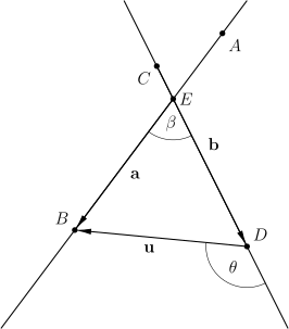
From the figure, \(|\mathbf a\times \mathbf b|=|\mathbf a||\mathbf b|\sin \beta\), \(|\mathbf u\times \mathbf b|=|\mathbf u||\mathbf b|\sin \theta\).
Taking the ratio:
It can be seen that \(\left|\dfrac{|\mathbf u|\sin \theta}{\sin \beta}\right|=l\). If the expression inside the absolute value is positive, it means translation along \(\mathbf a\); otherwise, it is in the opposite direction.
Moreover, multiplying \(T\) directly by \(\mathbf a\) automatically yields the unit vector of the line, eliminating the need for additional operations.
Thus, simply subtract \(T\mathbf a\) from point \(B\) to obtain the intersection.
Calculating Perimeter and Area of Arbitrary Polygons
Perimeter of an Arbitrary Polygon
Direct calculation suffices; simplicity is a virtue.
Area of an Arbitrary Polygon
Consider the geometric meaning of the magnitude of the cross product; we can use the cross product for this.
Label the polygon vertices counterclockwise as \(p_1,p_2,\cdots ,p_n\), and choose an auxiliary point \(O\). Define vectors \(\mathbf v_i=p_i-O\). Then the area \(S\) of the polygon is:
Circle-Line Related Problems
Intersection of a Line and a Circle
First, determine the positional relationship between the line and the circle. If they are disjoint, there is no intersection. If they are tangent, the tangent point can be found using the tangent line and the radius line, then reduced to finding the intersection of two lines.
If there are two intersections, the midpoint can be found using the Pythagorean theorem, then add/subtract half the chord length along the line direction.
Intersection of Two Circles
First, determine the positional relationship between the two circles. If they are externally disjoint or one contains the other, there is no intersection. If they are tangent, compute the direction vector of the line connecting the centers, then use the radii to compute the translation distance, and finally translate one center along this direction vector.
If the circles intersect, there are exactly two intersection points, symmetric about the line connecting the centers. Therefore, only one intersection point is described below; the other can be found similarly.
Connect one center to an intersection point, and compute the angle between this line and the line connecting the centers. Rotating the direction vector of the line connecting centers by this angle gives the direction vector of the radius from the center to the intersection point. Translating the center along this direction vector by the radius length yields one intersection point.
Polar Angle Sorting
Generally, such problems require first choosing a pole, then computing polar coordinates for other points, and solving the problem by sorting points by polar angle in the polar coordinate system.
「JOISC 2014 Day4」Two People's Constellations
There are \(n\) points in the plane, each colored with one of three colors. Count the number of pairs of non-intersecting triangles with three distinct colors. \(6\le n\le 3000\).
Solution
If two triangles do not intersect, there must exist two internal common tangents. If they intersect or one contains the other, internal common tangents do not exist. Common tangents of triangles are analogous to common tangents of circles.
First, choose an origin \(O\). Use this point as the pole and the horizontal line through it as the polar axis to establish a polar coordinate system. Sort the remaining points by polar angle from smallest to largest. Then count the number of points of each color above and below the polar axis.
Next, enumerate common tangents based on points. Let the enumerated point be \(P\), with the initial common tangent being the polar axis. Start counting. There must be a common tangent passing through \(O\) and \(P\). Since the common tangent does not intersect the triangles, one triangle chooses points above the tangent, and the other must choose points below. Then use the multiplication principle to count the number of valid pairs.
After counting, rotate the common tangent. Point \(P\) will change its position relative to the tangent (above/below), while other points remain unchanged; only update its position information. Thus, each pair of triangles is counted \(4\) times because each common tangent is enumerated twice. The final answer should be divided by \(4\).
Analyze the time complexity. We enumerate an origin, then sort the remaining points and perform linear counting for each origin. Thus, the time complexity is \(O(n^2\log n)\).
Coding Considerations
Since computational geometry often involves double floating-point calculations, precision and performance issues arise.
Some problems, such as finding the area of a triangle with integer coordinates, can exploit integer-only calculations to avoid floating-point precision issues.
Since floating-point input and computation are slower than integers, be mindful of constant factors affecting runtime.
本页面最近更新:,更新历史
发现错误?想一起完善? 在 GitHub 上编辑此页!
本页面贡献者:OI-wiki
本页面的全部内容在 CC BY-SA 4.0 和 SATA 协议之条款下提供,附加条款亦可能应用