Top Tree

Self-Adjusting Top Tree

Introduction

Self-Adjusting Top Tree is a data structure proposed by Tarjan and Werneck in their 2005 paper Self-Adjusting Top Trees, based on Top Tree theory, for maintaining fully dynamic forests. It is abbreviated as SATT.

Self-Adjusting Top Tree can perform operations such as path modification/query, subtree modification/query, and non-local search on any tree in the forest.

Splay Tree is the foundation of SATT, but the Splay Tree used in SATT differs in details from the ordinary Splay (some extensions have been made).

Problem Introduction

Maintain a forest, supporting the following operations:

• Delete or add an edge, ensuring the forest remains a forest after the operation.
• Modify the weights of a simple path in a tree.
• Modify the weights of a subtree rooted at a node.
• Query the sum of weights of a simple path in a tree.
• Query the sum of weights of a subtree rooted at a node.

Tree Contraction

For any tree, we can apply tree contraction theory to contract it into a single edge.

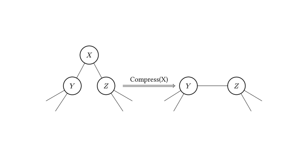
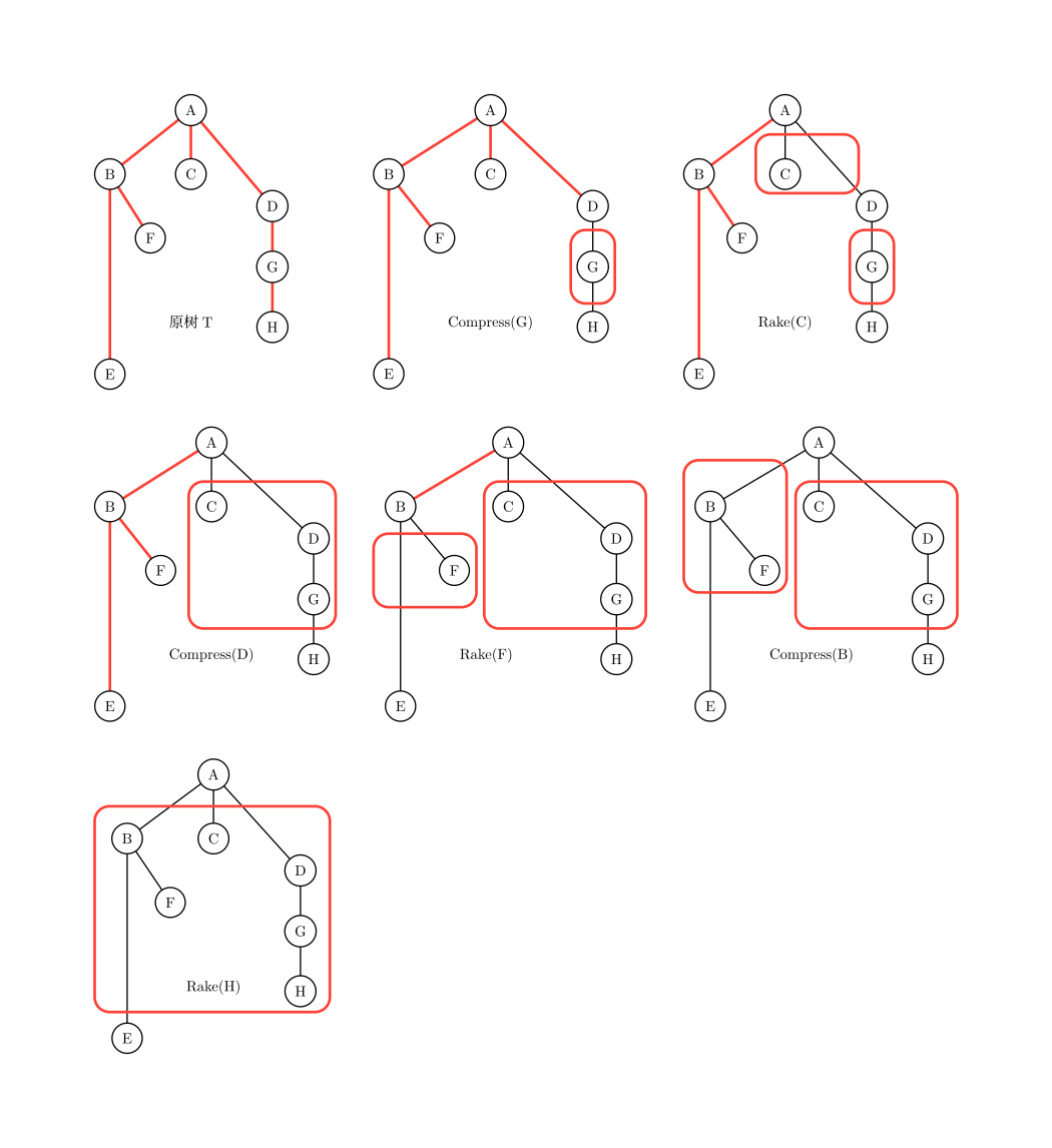
Specifically, tree contraction has two basic operations: Compress and Rake. The Compress operation specifies a node \(x\) with degree \(2\), with its two adjacent nodes denoted as \(y\) and \(z\). We add a new edge \(yz\); store the information of node \(x\), edge \(xz\), and edge \(xy\) in \(yz\), and then delete them. As shown in the figure.

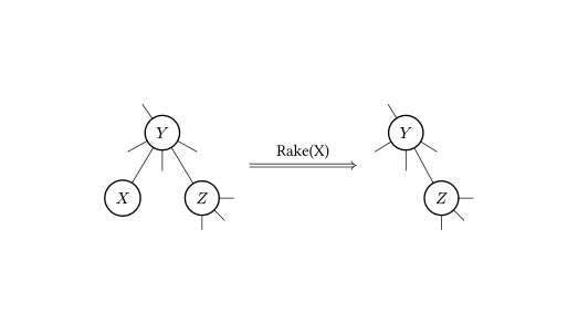
The Rake operation specifies a node \(x\) with degree \(1\), and the adjacent node \(y\) must have degree greater than \(1\). Let another neighbor of \(y\) be \(z\). We store the information of node \(x\) and edge \(xy\) into edge \(yz\), and then delete them. As shown in the figure.

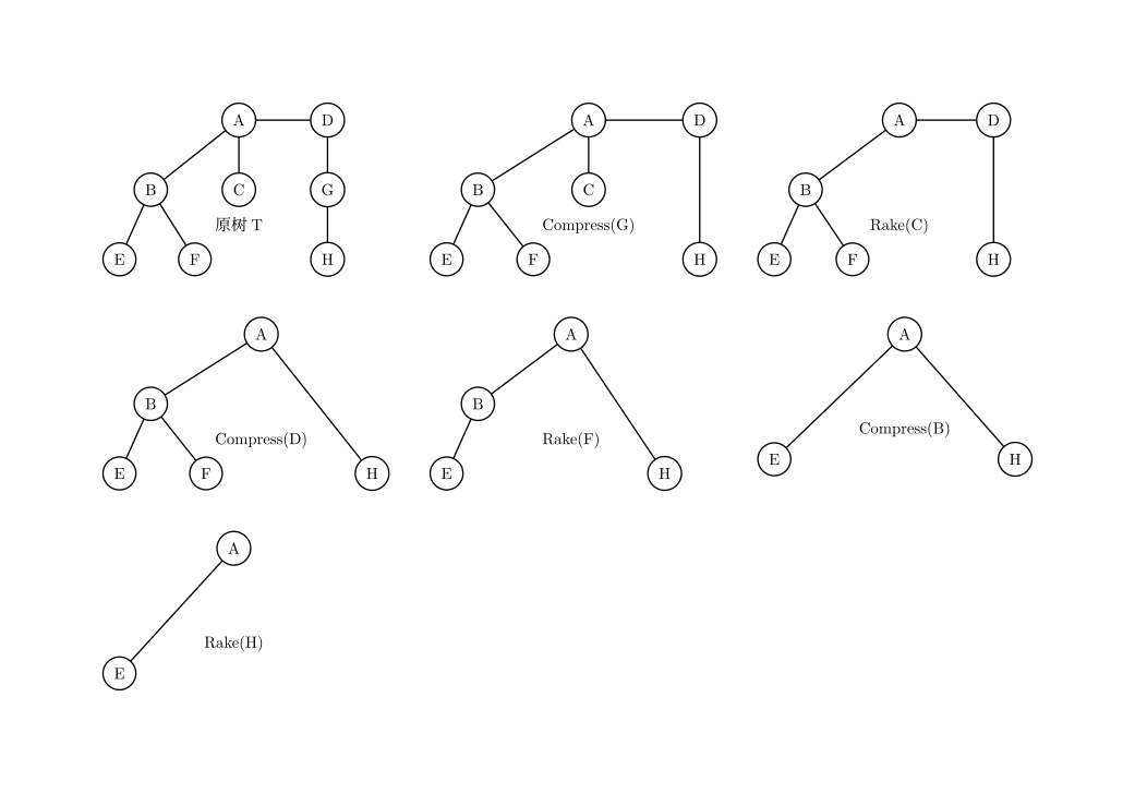
It can be proven that any tree can be contracted into a single edge using only Compress and Rake operations, as shown in the figure.

Cluster

For convenience, denote the original tree before any operations as \(T\). The tree after performing some tree contraction operations (possibly none) on \(T\) is denoted as \(T_x\).

We examine the information contained in a certain edge in some \(T_x\).

Besides its own information (if this edge does not exist in \(T\), it has no intrinsic information), this edge may also contain information from other points and edges merged onto it via Compress/Rake operations. Let's first select an edge from the tree contraction process in the figure below and see which points and edges in \(T\) its information represents.

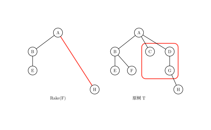
As shown, the selected edge and its corresponding subgraph are circled in red.

It can be seen that the points and edges represented by the information of this edge in \(T\) are connected. We can infer that for any edge in any \(T_x\), the stored information always corresponds to a connected subgraph in \(T\). We call such a connected subgraph a Cluster.

However, a cluster is an incomplete subgraph; it contains some edges whose endpoints are not included in the cluster itself. We call these endpoints the Endpoints of the cluster, the points of the connected subgraph it contains Internal Nodes, and the edges of the connected subgraph Internal Edges.

For any cluster, the following properties hold:

1. A cluster only stores and maintains information about internal nodes and internal edges.
2. A cluster has two endpoints. These two endpoints are the two points connected by the edge representing the cluster in \(T_x\). The path between the two endpoints is called the Cluster Path; denote the two endpoints of a cluster as \(x\) and \(y\), we use \(C(x,y)\) to represent this cluster.
3. Internal nodes are only connected to endpoints or other internal nodes.

In particular, each edge in \(T\) independently forms a cluster (containing only its own information), which we call a Base Cluster. For the final \(T_x\) contracted to a single edge, the edge represents a cluster containing all information of \(T\) except the two endpoints. This cluster is called the Root Cluster.

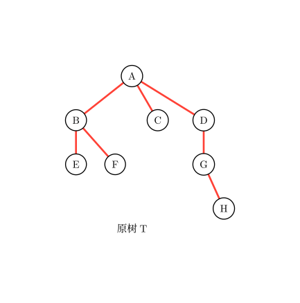
As shown, the base clusters mentioned above are marked with red lines.

From the perspective of clusters, Compress/Rake operations "merge" two clusters into one, leaving a new cluster. Thus, the tree contraction process is also the process of merging all base clusters into one cluster.

Therefore, we can also obtain the following figure, which is another representation of a series of tree contraction operations.

Top Tree

We now want to represent the entire tree contraction process for a given tree.

We can use the two methods mentioned above to represent this process, but this is cumbersome. If tree contraction takes \(n\) steps, we need \(n\) trees to represent the entire contraction.

Considering a more concise representation of a tree contraction for a given tree, we introduce the Top Tree.

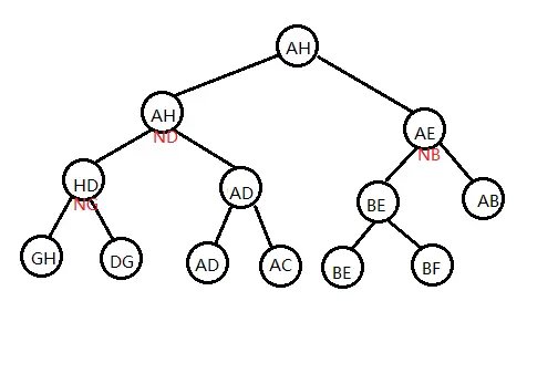
As shown, this is a Top Tree based on the contraction method and original tree described above.

Top Tree has the following properties:

1. A Top Tree corresponds to an original tree and a method of contracting it. Each node of the Top Tree represents an edge in some \(T_x\), i.e., a cluster formed during the tree contraction process. Points like \(N_x\) in the figure represent the cluster formed by the operation compress(x).
2. A node in the Top Tree has two children (each representing a cluster). The cluster represented by this node is the new cluster obtained by merging the two child clusters via Compress or Rake operations.
3. The leaf nodes of the Top Tree are base clusters, and its root node is the root cluster. Therefore, if we layer the Top Tree by its topological order, each layer represents a \(T_x\).

Information Maintenance Using Ternary Self-Adjusting Top Tree

Principle

The great simplification of the tree contraction process by Top Tree shows the possibility of maintaining tree information by maintaining the contraction process. SATT uses this principle to maintain tree information.

Note that the tree contraction process is also the process of gradually incorporating tree information. When we execute a compress(x), the information of point \(x\) starts to appear in some cluster from that moment, affecting our statistical results.

Suppose we now use a Top Tree to maintain a tree \(T\), where each point and edge has a weight, and we want to maintain the sum of weights of \(T\).

If we now modify the weight of a point \(x\) in \(T\) during maintenance, we obviously need to change the node information in the Top Tree for all clusters that include \(x\). Doing so would result in a single-operation time complexity of \(O(n)\).

However, if we choose a point such that the number of nodes in the Top Tree whose cluster information includes \(x\) is small—meaning its information is added to clusters as late as possible—the single-operation time complexity can be greatly improved. As shown in the figure.

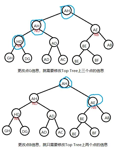
SATT maintains tree information by modifying the order in which information of a certain point/path is added to clusters during tree contraction (to reduce the single-operation time complexity when modified).

Actual Structure

First, we root the original tree \(T\) and assign layers. Then consider the root cluster of the Top Tree for a certain tree contraction order. It has two endpoints; we let one endpoint be the root of the original tree, and the other endpoint is arbitrarily chosen.

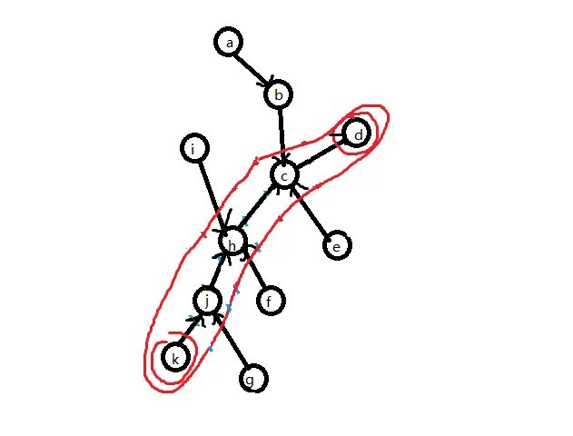
As shown, select a pair of endpoints for the root cluster; here endpoints are also circled when marking clusters.

From the basic operations of tree contraction, the information of points and edges on the cluster path \((j,h,c,jh,hc)\) is finally added to \(C(k,g)\) via Compress operations, while non-cluster-path points \((a,b,i,f,g,e,ig,\cdots)\) are added to \(C(k,g)\) via Rake operations.

We extract the cluster path separately; this is a tree with a special shape (a chain). We build a top tree for this tree (its represented tree contraction order is arbitrary).

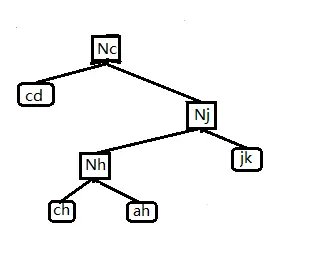
We call this structure Compress Tree, because in this Top Tree, any node's two children are merged into their parent via Compress operations.

Nodes in the Compress Tree are called Compress Nodes. Considering only the current cluster path, a non-leaf Compress Node represents a compress process, meaning merging the information of the left and right children, then adding the information of point \(x\) stored by compress(x) itself. This Compress Tree maintains the information of the cluster path of \(C(k,g)\).

Additionally, in the Compress Tree, we actually impose some restrictions on the Top Tree used. Note that the Compress Tree maintains a chain in \(T\) where the depths of points are all different. We stipulate that in the Compress Tree, the in-order traversal order of base clusters matches the depth order of the corresponding edges in \(T\), with smaller in-order traversal corresponding to shallower depth. Similarly, the same applies to the relationship for each point \(x\) corresponding to compress(x).

Now to maintain the information of those non-cluster paths, assume that points and edges on these non-cluster paths have already formed maximal clusters, and these maximal clusters are formed by Rake operations among smaller clusters circled in blue. For the process of merging several smaller clusters into a maximal cluster, we represent it with a ternary tree. Similarly, we call this structure Rake Tree, and correspondingly, points in the Rake Tree are Rake Nodes. Each Rake Node represents a cluster, formed by Raking its left and right children onto the smaller cluster represented by its middle child. See the figure below for details; note that each point in the Rake Tree represents a smaller cluster in \(T\) with the same endpoints.

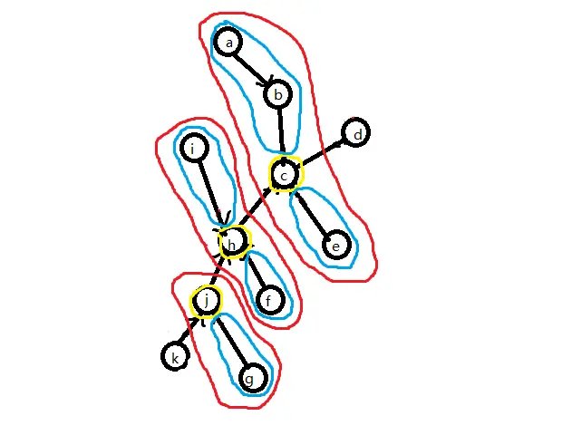
As shown, blue circles indicate maximal clusters, and yellow circles indicate smaller clusters.

For those smaller clusters, we process them similarly: select cluster paths, build Compress Trees, ... Recursively, we build many Compress Trees and Rake Trees representing tree contraction processes.

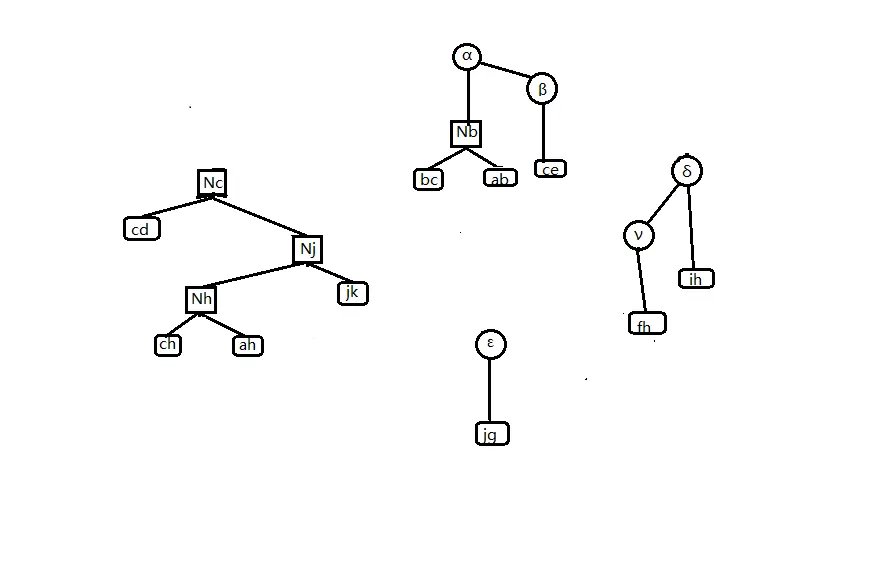
The above figure shows the Rake-Compress Tree of the original tree (since each Rake Node is connected to a Compress Tree, it appears as a Rake Tree connected to many Compress Trees) and the Compress Tree representing the root cluster path.

Consider concatenating these trees in some way to form an ordered whole. Denote the common endpoint of the set of minimal clusters represented by a Rake Tree as point \(x\). We add the other endpoint (not \(x\)) to the middle children of these Rake Nodes (a set of Compress Trees), while still maintaining their in-order traversal and basic properties of the Top Tree, as shown.

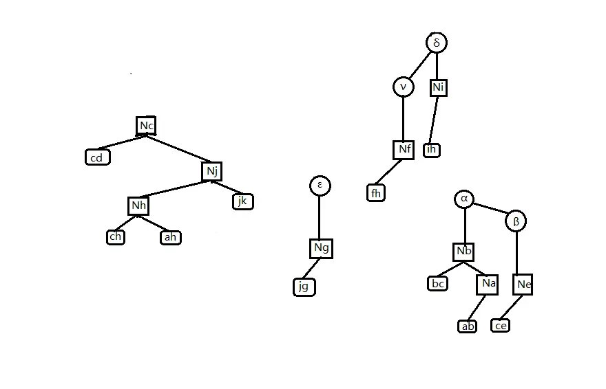
This step essentially allows the Rake operation that adds a point in \(T\) to occur directly in the Compress Tree. This not only enables correct maintenance of Rake Node information (just merge the three children's information) but also makes the Compress Tree structure more complete. Next, we modify the Compress Tree to a ternary tree. If the common endpoint of a Rake Tree is point \(x\), we attach the Rake Tree to the middle child of compress(x), as shown.

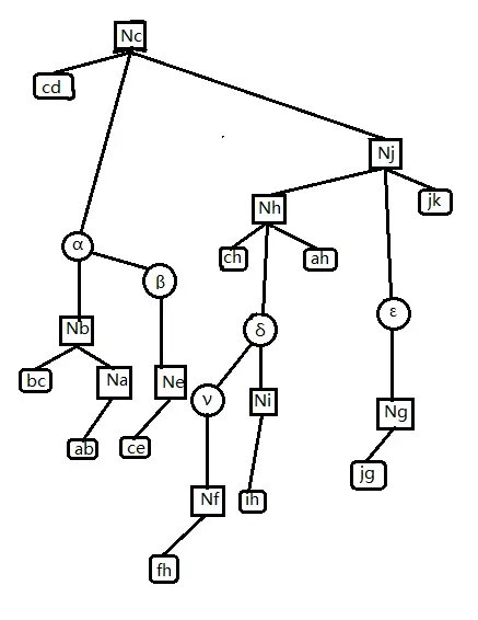
Now, after ternary transformation, the point compress(x) means: first Rake its middle child onto the cluster path, then combine the information of the left and right children and point \(x\).

Finally, we process the Compress Tree of the root cluster path: consistently with all other Compress Trees, add its two endpoints according to in-order traversal, so that its root stores the entire \(T\) information.

Thus, we achieve information maintenance of a tree using a ternary Self-Adjusting Top Tree.

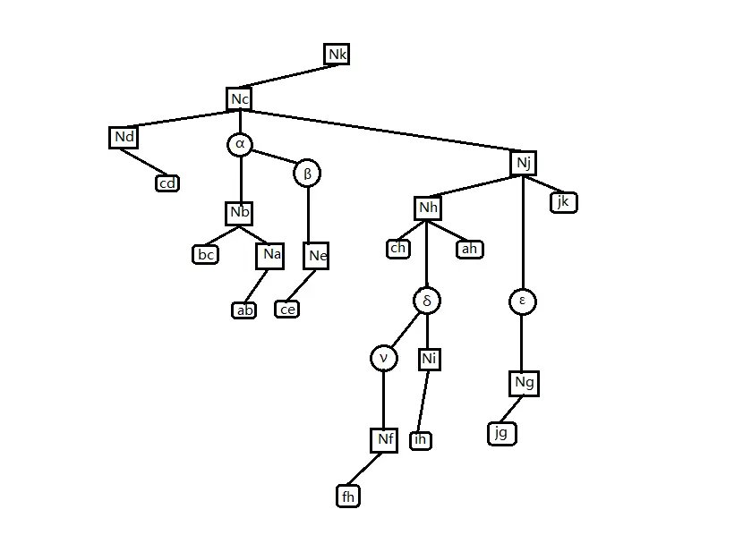
To summarize, SATT has the following properties:

1. SATT consists of Compress Trees and Rake Trees. A Compress Tree is a special Top Tree; a Rake Tree is a ternary tree. Both correspond to the tree contraction process of a tree.
2. A point in a Compress Tree has at most three children. Compress Trees can perform rotation operations similar to Splay Trees (just ensure the in-order traversal remains unchanged; when rotating a point, keep its middle child fixed).
3. A point in a Rake Tree always has a middle child. Rake Trees can perform rotation operations similar to Splay Trees (just ensure the in-order traversal remains unchanged; when rotating a point, keep its middle child fixed).
4. The topological order of SATT reflects the tree contraction order of the original tree \(T\).

Can SATT achieve "modifying the order in which information of a certain point/path is added to clusters during tree contraction" mentioned above? The answer is yes.

In SATT, there is an access(x) operation, whose purpose is to make point \(x\) become the non-root endpoint of the root cluster, while making compress(x) become the root of SATT.

We can use the access(x) operation with amortized \(O(\log n)\) complexity to rotate the point representing compress(x) in SATT to the root of the entire SATT. According to the fourth property of SATT, we change the operation order of compress(x), making it execute last, so the information of point \(x\) is added last. Thus, when we want to modify the information of point \(x\), we only need to update compress(x).

Code Implementation

Push Functions

First consider pushing up information, i.e., the Pushup(x) function. When maintaining information for a node in SATT, first discuss whether this node is in a Compress Tree or a Rake Tree, as explained above. Below we take maintaining the subtree size of a node as an example.

// ls(x) left child of x
// rs(x) right child of x
// ms(x) middle child of x
// type==0 is Compress Node
// type==1 is Rake Node
void pushup(int x, int type) {
  if (type == 0)
    size[x] = size[rs(x)] + size[ms(x)] + 1;
  else
    size[x] = size[rs(x)] + size[ms(x)] + size[ls(x)];
  return;
}

To query the subtree size of point \(x\), Access it to the SATT root; the answer is the size of its middle child \(+1\); because according to the above, after Access, its middle child is its true subtree.

Then consider pushing down information, i.e., the Pushdown(x) function. If we want to modify an entire subtree in the original tree, a natural idea is: Access the node to the SATT root, and mark its middle child. Similarly, query the subtree by Accessing and then querying the middle child.

If we want to modify an entire path in the original tree, we expose the two endpoints of the path, where expose(x, y) means making point \(x\) the root of \(T\), and point \(y\) the other endpoint of the root cluster. Correspondingly in SATT, the Compress Tree of the root cluster is the path from \(x\) to \(y\). Then directly mark the Compress Tree of the root cluster. Similarly, query the chain by exposing and then querying the root node.

Thus we know how to solve the problem introduced.

void pushdown(int x, int type) {
  if (type == 0) {
    // handle chain
    chain[ls(x)] += chain[x]; chain[rs(x)] += chain[x];
    val[ls(x)] += chain[x];
    val[rs(x)] += chain[x];
    // handle subtree
    subtree[ls(x)] += subtree[x];
    subtree[rs(x)] += subtree[x];
    subtree[ms(x)] += subtree[x];
    val[ls(x)] += subtree[x];
    val[rs(x)] += subtree[x];
    val[ms(x)] += subtree[x];
    subtree[x] = 0;
  } else {
    subtree[ls(x)] += subtree[x];
    subtree[rs(x)] += subtree[x];
    subtree[ms(x)] += subtree[x];
    val[ls(x)] += subtree[x];
    val[rs(x)] += subtree[x];
    val[ms(x)] += subtree[x];
    subtree[x] = 0;
  }
  return;
}

// push down all tags
void pushall(int x, int type) {
  if (!isroot(x)) pushall(father[x], type);
  pushdown(x, type);
  return;
}

Splay Functions

We know that Rake Trees and Compress Trees in SATT can be rotated, meaning they can be maintained with Splay. Therefore, we can write the following code:

// is a node's middle child or has no father
// ls left child of a SATT node
// rs right child of a SATT node
// ms middle child of a SATT node
// type==1 in Rake Tree
// type==0 in Compress Tree
bool isroot(int x) { return rs(father[x]) != x && ls(father[x]) != x; }

bool direction(int x) { return rs(father[x]) == x; }

void rotate(int x, int type) {
  int y = father[x], z = father[y], d = direction(x), w = son[x][d ^ 1];
  if (z) son[z][ms(z) == y ? 2 : direction(y)] = x;
  son[x][d ^ 1] = y;
  son[y][d] = w;
  if (w) father[w] = y;
  father[y] = x;
  father[x] = z;
  pushup(y, type);
  pushup(x, type);
  return;
}

void splay(int x, int type, int goal = 0) {
  pushall(x, type);  // push down tags
  for (int y; y = father[x], (!isroot(x)) && y != goal; rotate(x, type)) {
    if (father[y] != goal && (!isroot(y))) {
      rotate(direction(x) ^ direction(y) ? x : y, type);
    }
  }
  return;
}

Note that the functions direction and isroot differ from ordinary Splay. Because no matter how this point rotates, its middle child does not change.

Access Functions

access(x) means: rotate point \(x\) to the root of the entire SATT, making point \(x\) one of the two endpoints of the root cluster (the other endpoint is the root of \(T\)), without changing the structure of the original tree and the root of the original tree.

To implement access(x), we first rotate it to the root of its Compress Tree, then remove the right child of point \(x\), making point \(x\) an endpoint of the cluster corresponding to its Compress Tree.

if (rs(x)) {
  int y = new_node();
  setfather(ms(x), y, 0);
  setfather(rs(x), y, 2);
  rs(x) = 0;
  setfather(y, x, 2);
  pushup(y, 1);
  pushup(x, 0);
}

If point \(x\) has reached the root, exit; if not, perform the following steps to let it cross the Rake Tree above it:

1. Splay its parent node (must be a Rake Node) to the root of its Rake Tree.
2. Splay \(x\)'s grandparent node (must be a Compress Node) to the root of its Compress Tree.
3. If the grandparent node has a right child, swap point \(x\) with the grandparent's right child, update information, then exit.
4. If the grandparent node has no right child, first make point \(x\) the right child of the grandparent. At this point, \(x\)'s original parent node has no middle child; according to the properties of Rake Node, it cannot exist. So call the Delete function to delete it, then exit.

Steps 1 and 2 together are called Local Splay. Steps 3 and 4 together are called Splice. For convenience, we write them both in the Splice(x) function.

The Delete(x) function mentioned above is as follows:

1. Check if the point \(x\) to be deleted has a left child. If so, rotate the left child's subtree to below point \(x\) (becoming the new left child), then make the right child (if any) the right child of the left child. Now the left child replaces point \(x\). This is equivalent to a merge operation in Splay.
2. If there is no left child, directly let its right child replace point \(x\).

It is not hard to see that Splice(x) changes the endpoint selection of some clusters in the original tree. After one splice, we treat point \(x\)'s parent as the new point \(x\) and perform the next splice.

Eventually, we find that the point \(x\) we initially operated on must be at the far right of the Compress Tree of the root cluster. We just need to perform a final Global Splay to rotate it to the SATT root.

// ls left child of a SATT node
// rs right child of a SATT node
// ms middle child of a SATT node
// son[x][0] ls
// son[x][1] rs
// son[x][2] ms
// type==1 in Rake Tree
// type==0 in Compress Tree
int new_node() {
  if (top) {
    top--;
    return Stack[top + 1];
  }
  return ++tot;
}

void setfather(int x, int fa, int type) {
  if (x) father[x] = fa;
  son[fa][type] = x;
}

void Delete(int x) {
  setfather(ms(x), father[x], 1);
  if (ls(x)) {
    int p = ls(x);
    pushdown(p, 1);
    while (rs(p)) p = rs(p), pushdown(p, 1);
    splay(p, 1, x);
    setfather(rs(x), p, 1);
    setfather(p, father[x], 2);
    pushup(p, 1);
    pushup(father[x], 0);
  } else
    setfather(rs(x), father[x], 2);
  Clear(x);
}

void splice(int x) {
  // local splay
  splay(x, 1);
  int y = father[x];
  splay(y, 0);
  pushdown(x, 1);
  // splice
  if (rs(y)) {
    swap(father[ms(x)], father[rs(y)]);
    swap(ms(x), rs(y));
  } else
    Delete(x);
  pushup(x, 1);
  pushup(y, 0);
}

void access(int x) {
  splay(x, 0);
  if (rs(x)) {
    int y = new_node();
    setfather(ms(x), y, 0);
    setfather(rs(x), y, 2);
    rs(x) = 0;
    setfather(y, x, 2);
    pushup(y, 1);
    pushup(x, 0);
  }
  while (father[x]) {
    splice(father[x]);
    x = father[x];
    pushup(x, 0);
  }
  splay(x, 0);  // global splay
}

To make a point the root of the original tree, we Access point \(x\) to the root of SATT. At this point, \(x\) is already an endpoint of the final cluster. By the in-order traversal property of Compress Tree, swapping left and right children (swap left and right sons of all points) of the Compress Tree where point \(x\) is located makes point \(x\) the root of the original tree. In implementation, we achieve this by marking point \(x\) with a reversal tag and later pushing it down.

void makeroot(int x) {
  access(x);
  push_rev(x);
}

Thus expose(x, y) is straightforward:

void expose(int x, int y) {
  makeroot(x);
  access(y);
}

Link & Cut

Now we want to add an edge between two disconnected points in the original tree. First, make one point \(x\) the root of the original tree, then rotate the other point \(y\) to the root. At this point, point \(y\) should become the right child of point \(x\). Then attach this edge to the right child of point \(y\) (in SATT that only maintains points, this step can be omitted).

void Link(int x, int y, int z) {
  // z represents the edge connecting x, y
  access(x);
  makeroot(y);
  setfather(y, x, 1);
  setfather(z, y, 0);
  pushup(x, 0);
  pushup(y, 0);
}

Cut is similar in principle to Link.

void cut(int x, int y) {
  expose(x, y);
  clear(rs(x));  // delete the base cluster xy
  father[x] = ls(y) = rs(x);
  pushup(y, 0);
}

Complete Code

Luogu P3690【Template】Dynamic Tree

#include <iostream>
#define ls(x) T[x][0]
#define rs(x) T[x][1]
#define ms(x) T[x][2]
using namespace std;

constexpr int MAXN = 300005;

int T[MAXN][3], s[MAXN][2], tot, v[MAXN], r[MAXN], top, st[MAXN], f[MAXN];

int nnd() {
  if (top) {
    top--;
    return st[top + 1];
  }
  return ++tot;
}

bool isr(int x) { return rs(f[x]) != x && ls(f[x]) != x; }

bool dir(int x) { return rs(f[x]) == x; }

void psu(int x, int ty) {
  if (ty) {
    s[x][1] = s[ls(x)][1] ^ s[rs(x)][1] ^ s[ms(x)][1];
    return;
  }
  s[x][0] = s[ls(x)][0] ^ v[x] ^ s[rs(x)][0];
  s[x][1] = s[ls(x)][1] ^ s[ms(x)][1] ^ s[rs(x)][1] ^ v[x];
}

void psr(int x) {
  if (!x) return;
  r[x] ^= 1;
  swap(ls(x), rs(x));
}

void psd(int x, int ty) {
  if (ty) return;
  if (r[x]) {
    psr(ls(x));
    psr(rs(x));
    r[x] = 0;
  }
}

void upd(int x, int ty) {
  if (!isr(x)) upd(f[x], ty);
  psd(x, ty);
}

void stf(int x, int fa, int ty) {
  if (x) f[x] = fa;
  T[fa][ty] = x;
}

void rtt(int x, int ty) {
  int y = f[x], z = f[y], d = dir(x), w = T[x][d ^ 1];
  if (z) T[z][ms(z) == y ? 2 : dir(y)] = x;
  T[x][d ^ 1] = y;
  T[y][d] = w;
  if (w) f[w] = y;
  f[y] = x;
  f[x] = z;
  psu(y, ty);
  psu(x, ty);
}

void spy(int x, int ty, int gl = 0) {
  upd(x, ty);
  for (int y; y = f[x], (!isr(x)) && y != gl; rtt(x, ty)) {
    if (f[y] != gl && (!isr(y))) rtt(dir(x) ^ dir(y) ? x : y, ty);
  }
}

void cle(int x) {
  ls(x) = ms(x) = rs(x) = s[x][0] = s[x][1] = r[x] = v[x] = 0;
  st[++top] = x;
}

void del(int x) {
  stf(ms(x), f[x], 1);
  if (ls(x)) {
    int p = ls(x);
    psd(p, 1);
    while (rs(p)) p = rs(p), psd(p, 1);
    spy(p, 1, x);
    stf(rs(x), p, 1);
    stf(p, f[x], 2);
    psu(p, 1);
    psu(f[x], 0);
  } else
    stf(rs(x), f[x], 2);
  cle(x);
}

void spl(int x) {
  spy(x, 1);
  int y = f[x];
  spy(y, 0);
  psd(x, 1);
  if (rs(y)) {
    swap(f[ms(x)], f[rs(y)]);
    swap(ms(x), rs(y));
    psu(x, 1);
  } else
    del(x);
  psu(rs(y), 0);
  psu(y, 0);
}

void acs(int x) {
  spy(x, 0);
  int ys = x;
  if (rs(x)) {
    int y = nnd();
    stf(ms(x), y, 0);
    stf(rs(x), y, 2);
    rs(x) = 0;
    stf(y, x, 2);
    psu(y, 1);
    psu(x, 0);
  }
  while (f[x]) {
    spl(f[x]);
    x = f[x];
  }
  spy(ys, 0);
}

int fdr(int x) {
  acs(x);
  psd(x, 0);
  while (ls(x)) x = ls(x), psd(x, 0);
  spy(x, 0);
  return x;
}

void mkr(int x) {
  acs(x);
  psr(x);
}

void epo(int x, int y) {
  mkr(x);
  acs(y);
}

void lnk(int x, int y) {
  if (fdr(x) == fdr(y)) return;
  acs(x);
  mkr(y);
  stf(y, x, 1);
  psu(x, 0);
  psu(y, 0);
}

void cu(int x, int y) {
  epo(x, y);
  if (ls(y) != x || rs(x)) return;
  f[x] = ls(y) = 0;
  psu(y, 0);
}

int main() {
  cin.tie(nullptr)->sync_with_stdio(false);
  int n, m;
  cin >> n >> m;
  tot = n;
  for (int i = 1; i <= n; i++) {
    cin >> v[i];
    psu(i, 0);
  }
  for (int i = 1; i <= m; i++) {
    int op, U, V;
    cin >> op >> U >> V;
    if (op == 0) {
      epo(U, V);
      cout << s[V][0] << '\n';
    }
    if (op == 1) lnk(U, V);
    if (op == 2) cu(U, V);
    if (op == 3) {
      acs(U);
      v[U] = V;
      psu(U, 0);
    }
  }
  return 0;
}

Time Complexity Proof of SATT

Let the potential function for the current state \(x\) of a SATT (with \(n\) nodes) be

\[ \varphi(x)= \sum_{i=1}^{n} r(i) \]

where \(r(i) = \lceil \log_2 \text{siz}(i) \rceil\). \(\text{siz}(i)\) is the size of the subtree rooted at \(i\).

Then the amortized complexity of splay in SATT is clearly still \(3n\log n + 1\), even though SATT is a ternary tree.

Therefore, for SATT, as long as we prove the complexity of the Access function is correct, we prove the time complexity of SATT.

We analyze the amortized complexity of Access step by step.

First, we rotate point \(x\) to the root of its Compress Tree. The amortized complexity of this step is

\[ a \leq 3\log n +1 \]

Next, we make point \(x\) have no right child. The amortized complexity of this step is

\[ a = 1 + r'(\gamma)- 0 \leq \log n +1 \]

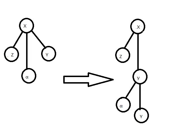
As shown, the process of removing the right child of point \(x\).

Then the process of alternating Local Splay and Splice. After several Splices, point \(x\) is rotated to the root of SATT. We analyze one set of Local Splay and Splice:

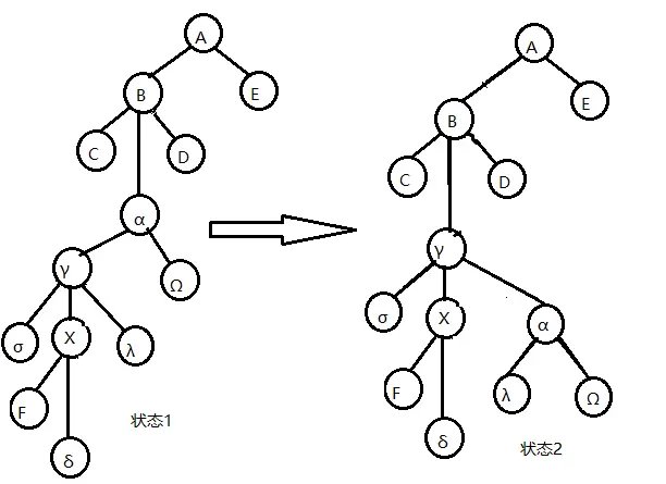
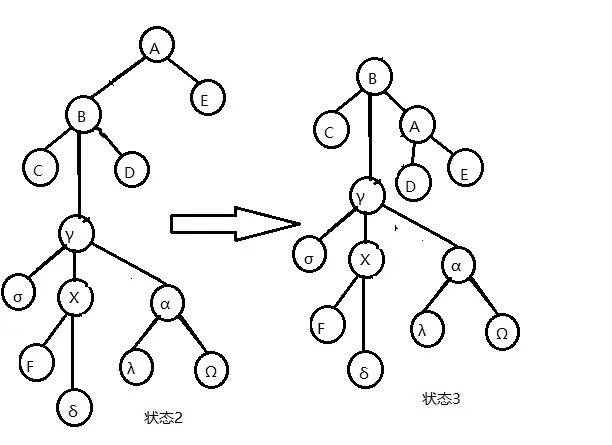
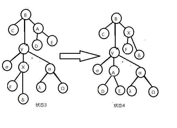
As shown, illustrates the process of performing one Splice on point \(x\), excluding the final left rotation of point \(x\).

For convenience, let \(r_x(i)\) be the \(r\) value of point \(i\) in state \(x\).

From the figure, it is easy to see that the amortized complexity of the operation from state 1 to state 2 (Local Splay rotating point \(x\)'s parent to the root of its Rake Tree) is

\[ a \leq 3(r_2(\gamma)- r_1(\gamma))+1 \]

From the figure, the amortized complexity of the operation from state 2 to state 3 (Local Splay rotating point \(x\)'s grandparent to the root of its Compress Tree) is

\[ a \leq 3(r_3(B)- r_2(B))+1 \]

Focus on the operation from state 3 to state 4 (Splice)

\[ a = r_4(\gamma) -r_3(\gamma) +1 \]

It is not hard to see \(r_4(\gamma) \leq r_3(B)\)

Thus the amortized complexity of this operation is

\[ \begin{aligned} a &\leq r_3(B)- r_3(\gamma)+1\\ &\leq 3(r_3(B)- r_3(\gamma))+1\\ \end{aligned} \]

Combining the above, the complexity of one Splice is

\[ a\leq 3r_3(B)+3r_3(B)+3r_2(\gamma)-3r_3(\gamma)-3r_2(B)-3r_1(\gamma)+3 \]

Denote the \(r\) value of the next Splice point \(X\) (point \(B\) in state 4) as \(r'(X)\), and note that \(r_3(\gamma),r_1(\gamma) \ge r_1(X)\), \(r_3(B),r_2(\gamma) \leq r'(X)\) and \(r_3(B)=r_2(B)\), so

\[ a\leq 9(r'(X)-r(X))+3 \]

Besides this complexity, there may be additional amortized complexity due to delete(x) in Splice, denote this part as \(a' \leq 3\log n +1\).

Ignoring \(a'\) for now, each Splice's \(r'(X)\) equals the next \(r(X)\), and the first Splice's \(r(X)\) equals the \(r(X)\) when we initially rotate point \(x\) to its Compress Tree root. Then for an access(x) without counting delete(x), we have:

\[ a \leq 9(r'(x)-r(x))+ 3k + 1 \]

where \(k\) is the number of Splices.

It seems \(a\) will have a \(3k+1\) term making amortized complexity hard to analyze, but we have a way to handle it. Note that zig-zig/zig-zag rotations can be amortized as

\[ \begin{aligned} a &\leq 3(r'(X)-r(X)) + q\\ &\leq 3(q-1)(r'(X)-r(X)) \end{aligned} \]

If we can find enough zig-zig, zig-zag operations, we can spread this \(3k+1\) over these operations, thus eliminating the \(3k+1\).

We find that Global Splay has many such zig-zig, zag-zig operations for us to use, because the number of points in Global Splay must be greater than \(k\), and the number of points on the path from point \(x\) to the root of Global Splay is at least \(k\). That means in one access(x), there will be at least \(\dfrac k2\) zig-zag operations. Including the amortized complexity of Global Splay \(a \leq 3\log n +1\), the amortized complexity of one access(x) without counting delete(x) is

\[ \begin{aligned} a&\leq 9(r'(X)-r(X)) + 3k + 1 + 18(r''(X)-r'(X)) -S+1 +3 \log n +1,S \ge 3k\\ a&\leq 18(r''(X)-r(X)) +2 +3\log n+1\\ a&\leq 21(r''(X)-r(X)) +3 \end{aligned} \]

Now including \(a'\), write the total expression for \(m\) access(x) operations.

\[ \sum_{i=1}^m a_i' + \sum_{i=1}^m a_i = \sum_{i=1}^m c_i + \varphi(x_n) -\varphi(x_0) \]

We want the actual complexity

\[ \begin{aligned} \sum_{i=1}^m c_i &= \sum_{i=1}^m a_i +\sum_{i=1}^m a_i' - \varphi(x_n) +\varphi(x_0)\\ &\le \sum_{i=1}^m a_i' + 21m\log n +n\log n +3m \end{aligned} \]

Note that the delete(x) operation essentially deletes a Rake Node, but in \(m\) operations we add at most \(m\) Rake Nodes. By the definition of Rake Node, initially we have at most \(n\) Rake Nodes, meaning we will perform at most \(m+n\) delete(x) operations. Since \(a' \leq 3\log n +1\), we have

\[ \sum_{i=1}^m c_i \leq 3(m+n)\log n + 21m\log n +n\log n +4m +n \]

Thus we have proven the complexity of Access, and since other functions are either based on Access or have constant time complexity, we have proven the complexity of SATT.

Incidentally, if we omit the Global Splay process like LCT, and instead directly rotate the point to be Accessed during each Splice, the time complexity is also correct (in practice, the version omitting Global Splay is much faster, comparable to LCT on Luogu P3690).

Example Problems

Example 1

CEOI 2019 Dynamic Diameter

Given a tree with \(n\) nodes, each edge has a weight. There are \(q\) updates, each modifying the weight of an edge, and querying the diameter of the tree. Forced online.

Maintain dynamic diameter. After building SATT, we only need to maintain the answer for each point in Pushup(x), and finally query the answer of the root node (i.e., the diameter of the entire tree).

void pushup(int x, int op) {
  if (op == 0) {
    // is Compress Node
    len[x] = len[ls(x)] + len[rs(x)];
    diam[x] = maxs[ls(x)][1] + maxs[rs(x)][0];
    diam[x] =
        max(diam[x], max(maxs[ls(x)][1], maxs[rs(x)][0]) + maxs[ms(x)][0]);
    diam[x] = max(diam[x], max(max(diam[ls(x)], diam[rs(x)]), diam[ms(x)]));
    maxs[x][0] =
        max(maxs[ls(x)][0], len[ls(x)] + max(maxs[ms(x)][0], maxs[rs(x)][0]));
    maxs[x][1] =
        max(maxs[rs(x)][1], len[rs(x)] + max(maxs[ms(x)][0], maxs[ls(x)][1]));
  } else {
    // is Rake Node
    diam[x] = maxs[ls(x)][0] + maxs[rs(x)][0];
    diam[x] =
        max(diam[x], maxs[ms(x)][0] + max(maxs[ls(x)][0], maxs[rs(x)][0]));
    diam[x] = max(max(diam[x], diam[ms(x)]), max(diam[ls(x)], diam[rs(x)]));
    maxs[x][0] = max(maxs[ms(x)][0], max(maxs[ls(x)][0], maxs[rs(x)][0]));
  }
  return;
}

Here \(diam\) is the answer of the current point (the diameter of the cluster represented by this point). \(len\) represents the length of the cluster path of the current Compress Node, \(maxs_{0/1}\) represents the maximum distance from the Compress Node to points and endpoints inside the cluster without choosing the cluster path child/without choosing the parent (if it's a Rake Node, only store \(maxs_0\), the maximum distance from the upper endpoint of the current cluster to points and endpoints inside the cluster). Each query asks for the diam of the SATT root node; correctness is obvious.

Note to modify Pushrev(x) accordingly.

```cpp void pushrev(int x) { if (!x) return; r[x] ^= 1; swap(ls(x), rs(x)); swap(maxs[x][0], maxs

---

本页面最近更新：，更新历史
发现错误？想一起完善？ 在 GitHub 上编辑此页！
本页面贡献者：OI-wiki
本页面的全部内容在 CC BY-SA 4.0 和 SATA 协议之条款下提供，附加条款亦可能应用