Linear Basis
Recall the concept of basis vectors in high school solid geometry. In three-dimensional Euclidean space, we can find a set of basis vectors \(\boldsymbol{i}\), \(\boldsymbol{j}\), \(\boldsymbol{k}\). After that, any vector in the space can be represented by these basis vectors. In other words, we can describe the infinite three-dimensional space through a finite set of basis vectors, which sufficiently demonstrates the importance of basis vectors.
Three-dimensional Euclidean space is a special linear space. The basis vectors of three-dimensional Euclidean space are generalized to linear bases in linear spaces.
In OI, applications related to linear bases generally only involve two types of linear spaces: the \(n\)-dimensional real linear space \(\mathbf{R}^n\) and the \(n\)-dimensional Boolean domain linear space \(\mathbf{Z}_2^n\). We will introduce them in detail in the Applications section. If you are not familiar with linear algebra, it is recommended to start reading from the applications section.
The following will introduce linear bases from the perspective of general linear spaces and present common properties of linear bases.
Prerequisite: Linear Space.
A linear basis is a basis of a linear space and an important tool for studying linear spaces.
Definition
A maximal linearly independent set of a linear space \(V\) is called a Hamel basis or linear basis of \(V\), simply referred to as a basis.
It is stipulated that the basis of the linear space \(\{\theta\}\) is the empty set.
It can be proven that any linear space has a linear basis1. We define the dimension of a linear space \(V\) as the number (or cardinality) of elements in its linear basis, denoted as \(\dim V\).
Properties
-
For a finite-dimensional linear space \(V\), let its dimension be \(n\), then:
-
Any \(n+1\) vectors in \(V\) are linearly dependent.
-
Any \(n\) linearly independent vectors in \(V\) form a basis of \(V\).
-
If any vector in \(V\) can be linearly expressed by the vector group \(a_1,a_2,\dots,a_n\), then it is a basis of \(V\).
Proof
Take any basis \(b_1,b_2,\dots,b_n\) of \(V\). By the given condition, the vector group \(b_1,b_2,\dots,b_n\) can be linearly expressed by \(a_1,a_2,\dots,a_n\), so
\[ n=\operatorname{rank}\{b_1,b_2,\dots,b_n\}\leq\operatorname{rank}\{a_1,a_2,\dots,a_n\}\leq n \]Therefore \(\operatorname{rank}\{a_1,a_2,\dots,a_n\}=n\).
-
Any linearly independent vector group \(a_1,a_2,\dots,a_m\) in \(V\) can be extended to a basis of \(V\) by inserting some vectors.
-
-
(Subspace Dimension Formula) Let \(V_1,V_2\) be finite-dimensional linear spaces over \(\Bbb{P}\), and \(V_1+V_2\) and \(V_1\cap V_2\) are also finite-dimensional, then \(\dim V_1+\dim V_2=\dim(V_1+V_2)+\dim(V_1\cap V_2)\).
Proof
Let \(\dim V_1=n_1\), \(\dim V_2=n_2\), \(\dim(V_1\cap V_2)=m\).
Take a basis \(a_1,a_2,\dots,a_m\) of \(V_1\cap V_2\), and extend it to bases of \(V_1\) and \(V_2\) respectively: \(a_1,a_2,\dots,a_m,b_1,b_2,\dots,b_{n_1-m}\) and \(a_1,a_2,\dots,a_m,c_1,c_2,\dots,c_{n_2-m}\).
Next, we only need to prove that the vector group \(a_1,a_2,\dots,a_m,b_1,b_2,\dots,b_{n_1-m},c_1,c_2,\dots,c_{n_2-m}\) is linearly independent.
Suppose \(\sum_{i=1}^m r_ia_i+\sum_{i=1}^{n_1-m} s_ib_i+\sum_{i=1}^{n_2-m} t_ic_i=\theta\).
Then \(\sum_{i=1}^{n_2-m} t_ic_i=-\sum_{i=1}^m r_ia_i-\sum_{i=1}^{n_1-m} s_ib_i\).
Note that the left side is in \(V_2\), and the right side is in \(V_1\), so both sides are in \(V_1\cap V_2\). Therefore, \(\sum_{i=1}^{n_2-m} t_ic_i=\sum_{i=1}^m k_ia_i\).
Hence \(t_1=t_2=\dots=t_{n_2-m}=k_1=k_2=\dots=k_m=0\), and then \(r_1=r_2=\dots=r_m=s_1=s_2=\dots=s_{n_1-m}=t_1=t_2=\dots=t_{n_2-m}=0\).
-
Let \(V_1,V_2\) be finite-dimensional linear spaces over \(\Bbb{P}\), and \(V_1+V_2\) and \(V_1\cap V_2\) are also finite-dimensional, then the following statements are equivalent:
-
\(V_1+V_2=V_1\oplus V_2\).
-
\(\dim V_1+\dim V_2=\dim(V_1+V_2)\).
-
If \(a_1,a_2,\dots,a_n\) is a basis of \(V_1\), and \(b_1,b_2,\dots,b_m\) is a basis of \(V_2\), then \(a_1,a_2,\dots,a_n,b_1,b_2,\dots,b_m\) is a basis of \(V_1+V_2\).
Note
Statements 1 and 3 can be generalized to infinite-dimensional linear spaces.
-
Examples
Consider bases of \(\Bbb{R}^2\).
-
As shown in the figure
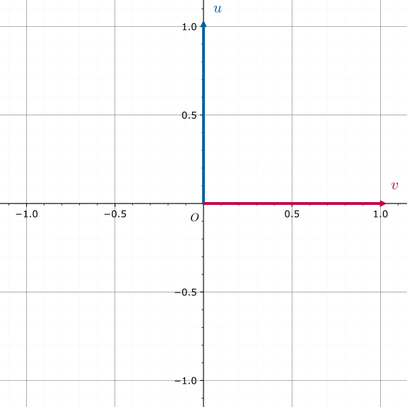
\(u,v\) form a basis.
-
As shown in the figure
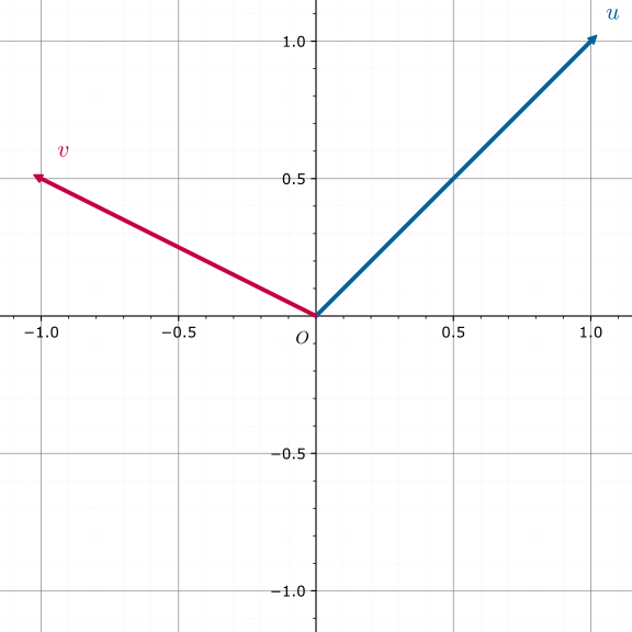
\(u,v\) form a basis.
-
As shown in the figure
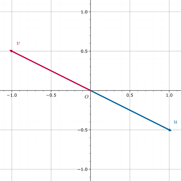
\(u,v\) do not form a basis because \(u=-v\).
-
As shown in the figure
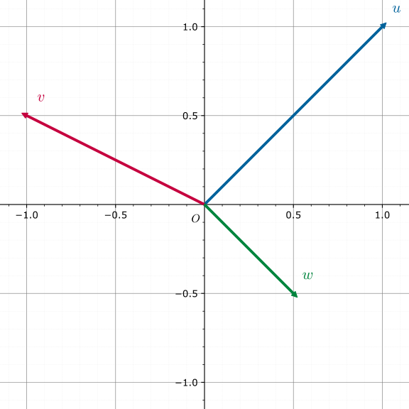
\(u,v,w\) do not form a basis because \(u+4v+6w=\theta\).
Orthogonal Basis and Orthonormal Basis
If a basis \(B\) of a linear space \(V\) satisfies \(\forall b,b'\in B,~(b,b')\ne 0\iff b=b'\) (i.e., pairwise orthogonal), then this basis is called an orthogonal basis.
If an orthogonal basis \(B\) of a linear space \(V\) also satisfies \(\forall b\in B,~|b|=\sqrt{(b,b)}=1\), then this basis is called an orthonormal basis.
Any basis of a finite-dimensional linear space \(V\) can be transformed into an orthogonal basis via Schmidt orthogonalization.
Applications
Based on the previous content, we can use linear bases to achieve:
- Find the rank of a given set of vectors;
- For a given set of vectors, find a maximal linearly independent subset (or a basis of the linear space they span);
- Insert certain vectors into a given set of vectors, and find a maximal linearly independent subset (or a basis of the linear space they span) after insertion;
- For a found maximal linearly independent subset (or basis), determine whether a vector can be linearly expressed by it;
- For a found maximal linearly independent subset (or basis), find special elements in the spanned linear space (such as maximum, minimum, etc.).
In OI, we generally refer to the linear basis under the \(n\)-dimensional real linear space \(\mathbf{R}^n\) as the real linear basis, and the linear basis under the \(n\)-dimensional Boolean domain linear space \(\mathbf{Z}_2^n\) as the XOR linear basis.
Tip
In \(\mathbf{Z}_2\), addition is XOR, and multiplication is AND. It can be proven that \(\mathbf{Z}_2\) is a field.
It can be proven that the algebraic system \((\mathbf{Z}_2^n,+,\cdot,\mathbf{Z}_2)\) is a linear space, where:
That is, addition is XOR, and scalar multiplication is AND.
Taking the XOR linear basis as an example, we can construct an XOR linear basis \(B=\{b_1,\dots,b_n\}\) from a given set of Boolean sequences \(\{x_1,\dots,x_m\}\). This basis has the following properties:
- The XOR sum of any non-empty subset of \(B\) is not \(0\);
- For any element \(x\) in \(X\), we can take some elements from \(B\) such that their XOR sum is \(x\);
- For any set \(B'\) satisfying the above two conditions, its number of elements is not less than that of \(B\).
We can use the XOR linear basis to achieve:
- Determine whether a number can be expressed as the XOR sum of a subset of a given set of numbers;
- Find the number of ways to express a number as the XOR sum of a subset of a given set of numbers;
- Find the maximum/minimum/k-th largest/k-th smallest XOR sum of subsets of a given set of numbers;
- Find the rank of a number among the XOR sums of subsets of a given set of numbers.
Construction Methods
Since XOR linear bases and real linear bases are essentially the same, the following uses XOR linear bases as an example. The code for the real linear basis version only requires simple modifications.
Greedy Method
For each number \(p\) in the original set, convert it to binary, and scan from the highest bit to the lowest bit. For the \(x\)-th bit being \(1\), if \(a_x\) does not exist, then set \(a_x \leftarrow p\) and stop scanning; if it exists, set \(p\leftarrow p~\text{xor}~a_x\).
To query the maximum XOR sum of any several elements in the original set, simply scan the linear basis from the highest bit to the lowest bit. If XORing with the current \(a_x\) increases the answer, then XOR the answer with \(a_x\).
Why does this work? Because scanning from high to low bits, if the current bit is the \(i\)-th bit, it means we can ensure the \(i\)-th bit of the answer is \(1\), and there is no chance to change the \(i\)-th bit later.
To query the minimum XOR sum of any several elements in the original set, it is the smallest element among all elements in the linear basis set.
To query whether a number can be XORed out, it is similar to insertion. If the last inserted number \(p\) is XORed to \(0\), then it can be XORed out.
Code (Luogu P3812 【Template】Linear Basis)
1 2 3 4 5 6 7 8 9 10 11 12 13 14 15 16 17 18 19 20 21 22 23 24 25 26 27 28 29 30 31 32 33 34 35 36 | |
Gaussian Elimination Method
The Gaussian elimination method constructs a linear basis from the perspective of linear equations, and its correctness is obvious.
Code (Luogu P3812 【Template】Linear Basis)
1 2 3 4 5 6 7 8 9 10 11 12 13 14 15 16 17 18 19 20 21 22 23 24 25 26 27 28 29 30 31 32 33 34 35 36 37 38 39 | |
Properties
The linear basis constructed by the greedy method has the following properties:
- The linear basis has no subset with XOR sum \(0\).
- The highest binary bits of the numbers in the linear basis are different.
The linear basis constructed by Gaussian elimination satisfies the following property:
-
The matrix after Gaussian elimination is a row-reduced echelon matrix.
This property includes the two properties satisfied by the linear basis constructed by the greedy method.
If you do not understand the correctness of this property, you can jump to Gaussian Elimination.
Provide a sample set:
1 2 | |
Binary representation:
1 2 3 4 5 | |
Linear basis generated by the greedy method:
1 2 3 4 5 6 7 8 9 10 | |
Linear basis generated by Gaussian elimination:
1 2 3 4 5 6 7 8 9 10 | |
This is a very good property that helps us solve many problems more conveniently. For example: given some numbers, select some of them to XOR, and find the maximum XOR value. If using the greedy method to construct the linear basis, we need to perform the greedy process again. If the current bit of ans is 0, then XORing will definitely be better; otherwise, if the current bit is 1, it will definitely not be better. However, after constructing the linear basis using Gaussian elimination, we can directly XOR all elements in the linear basis and output the result.
For other classic problems (query whether a number can be XORed out, query the \(k\)-th largest number that can be XORed out, etc.), the linear basis obtained by Gaussian elimination can also be solved more conveniently.
Time Complexity
Let the vector length be \(n\) and the total number be \(m\). Then the time complexity is \(O(nm)\). The constant of Gaussian elimination is slightly larger.
For real linear bases, the time complexity is \(O(n^2m)\).
Linear Basis Merging
Merging linear bases only requires brute force processing, i.e., inserting one set of linear bases into another set of linear bases. The time complexity of a single merge is \(O(n^2)\) (for XOR linear bases) or \(O(n^3)\) (for real linear bases).
Linear Basis Intersection
Linear basis intersection, strictly speaking, is to find a linear basis of the intersection space of the two linear spaces they span. This section introduces two algorithms. The time complexity of a single intersection for both algorithms is \(O(n^2)\) (for XOR linear bases) or \(O(n^3)\) (for real linear bases).
Naive Algorithm
Let the linear bases to be intersected be \(\alpha\) and \(\beta\). The algorithm for linear basis intersection only requires the following adjustments to the brute force merging algorithm for linear bases (taking XOR linear bases as an example):
- Use the Greedy Method to attempt to insert each vector \(\beta_j\) from linear basis \(\beta\) into \(\alpha\), and initialize the intersection linear basis \(\gamma\) as an empty set;
- During insertion, record the contribution of elements from linear basis \(\beta\) in the vector to be inserted. Specifically, maintain a new vector \(b\), initialized as \(\beta_j\). Moreover, if the vector being inserted is XORed with the vector at position \(x\) in the linear basis, then the contribution \(b\) should also be XORed with the contribution \(b_x\) recorded at position \(x\);
- If the insertion is successful, and vector \(\beta_j'\) is inserted at position \(x\) of the linear basis, change the recorded \(b_x\) at position \(x\) to the contribution \(b\) from elements of linear basis \(\beta\) during the process of obtaining \(\beta_j'\);
- If the insertion fails, insert the recorded contribution \(b\) from elements of linear basis \(\beta\) during the process into \(\gamma\).
The resulting linear basis \(\gamma\) is the desired intersection. Of course, this algorithm also computes the union of the linear bases simultaneously.
Explanation of the Algorithm
Let the merged linear basis be \(\{\alpha_1,\cdots,\alpha_m,\beta'_{j_1},\cdots,\beta'_{j_\ell}\}\), where \(\beta'_{j_k}\) is the final vector obtained when inserting \(\beta_{j_k}\). Then, \(\{\alpha_1,\cdots,\alpha_m,\beta_{j_1},\cdots,\beta_{j_\ell}\}\) is also a merged linear basis. Denote \(\beta^+\) as the set \(\{\beta_{j_1},\cdots,\beta_{j_\ell}\}\). Then the merged basis can be written as \(\alpha\cup\beta^+\). Moreover, each vector \(c\) in the sum space can be uniquely expressed as
where \(a\in\operatorname{span}\alpha\) and \(b\in\operatorname{span}\beta^+\). The \(b\) in this decomposition is exactly what the previous algorithm attempts to record as the "contribution of elements from linear basis \(\beta\)". Strictly speaking, it is only the contribution of those vectors from \(\beta\) that were successfully inserted last.
For successful insertions, the final recorded \(b\) is the \(b\) term in this decomposition. Let \(\beta_j\in\beta^+\). Initially, \(\beta_j=0\oplus\beta_j\), which is already the correct decomposition of \(\beta_j\) on the basis \(\alpha\cup\beta^+\). When updating \(\beta'_j=a\oplus b\) to \(\beta'_j\oplus c_x\), since \(\beta_j'\oplus c_x=(a\oplus a_x)\oplus(b\oplus b_x)\), we only need to update \(b\) to \(b\oplus b_x\) to ensure the decomposition remains correct. Therefore, by induction, when finally inserting \(\beta'_j\) into the merged linear basis, the recorded contribution \(b\) is the \(b\) term in the above decomposition.
For unsuccessful insertions, the variable to be inserted will eventually become \(0\), and the contribution \(b\) at this time should be inserted into \(\gamma\). At this point, if we repeat the above argument, we will find that we can still guarantee \(\beta_j'=a\oplus b\) during the insertion process, with \(a\in\operatorname{span}\alpha\), but \(b\) no longer belongs to \(\operatorname{span}\beta^+\). This is because initially, in \(\beta_j=0\oplus\beta_j\), we have \(\beta_j\notin\beta^+\). Apart from that, the terms XORed during contribution updates all belong to \(\operatorname{span}\beta^+\). So, actually, we have \(b\oplus\beta_j\in\operatorname{span}\beta^+\).
Then, why does inserting all these \(b\) from unsuccessful insertions into \(\gamma\) yield a linear basis of the intersection space? First, if inserting \(\beta_j\) fails, we will eventually get \(0=a\oplus b\), where \(a\in\operatorname{span}\alpha\) and \(b\in\operatorname{span}(\beta^+\cup\{\beta_j\})\subseteq\operatorname{span}\beta\). Therefore, \(b=a\) must lie in the intersection space \(\operatorname{span}\alpha\cap\operatorname{span}\beta\). Conversely, let \(c\) be any element in the intersection space. Since \(c\in\operatorname{span}\beta\), \(c\) can be expressed as a linear combination (XOR sum) of elements in \(\beta\):
where \(\lambda_j\in\{0,1\}\). For each \(\beta_j\notin\beta^+\), denote the corresponding contribution inserted into \(\gamma\) as \(b_j\). Then we have
Note that both \(b_j\) and \(c\) lie in the intersection space, so the left side must also lie in the intersection space, and thus can be written as a linear combination of elements in \(\alpha\). Meanwhile, all terms on the right side are either \(\beta_j\in\beta^+\) or \(\beta_j\notin\beta^+\) with \(\beta_j\oplus b_j\in\beta^+\). Therefore, the right side is actually a linear combination of elements in \(\beta^+\). However, \(\alpha\cup\beta^+\) is linearly independent, so all coefficients are \(0\), meaning \(c=\bigoplus_{\beta_j\notin\beta^+}\lambda_jb_j\in\operatorname{span}\{b_1,\cdots,b_j\}\). This shows that these contributions \(b\) from vectors that cannot be inserted together span the intersection space.
According to this explanation, the purpose of maintaining the contribution \(b\) during the process is actually to maintain the decomposition \(a\oplus b\). Moreover, when finally inserting contributions into \(\gamma\), we always have \(a=b\). Therefore, whether we maintain the contribution of elements from \(\alpha\) or \(\beta\) (i.e., whether we maintain \(a\) or \(b\)), the result obtained is correct. If we want to maintain the contribution of elements from linear basis \(\alpha\), we only need to modify the initial values of the corresponding contributions: each vector \(\alpha_i\) in \(\alpha\) initially has contribution \(\alpha_i\), while the inserted \(\beta_j\) initially has contribution \(0\).
Template problem code:
Code (Library Checker Intersection of \(\mathbf F_2\) vector spaces)
1 2 3 4 5 6 7 8 9 10 11 12 13 14 15 16 17 18 19 20 21 22 23 24 25 26 27 28 29 30 31 32 33 34 35 36 37 38 39 40 41 42 43 44 45 46 47 48 49 50 51 52 53 54 55 56 57 58 59 60 61 62 63 64 65 66 67 68 69 70 71 72 73 74 75 76 77 78 79 80 81 82 83 84 85 86 87 88 89 | |
Zassenhaus Algorithm
Another equivalent approach is the Zassenhaus algorithm, which can also simultaneously compute the union and intersection of two linear bases. The complexity is exactly the same as above.
Specific steps are as follows:
- Initialize a linear basis \(\gamma\) with vector length \(2n\) as empty. The vectors are written in the form \((a,b)\), where both \(a\) and \(b\) have length \(n\);
- Insert each element \(\alpha_i\) from \(\alpha\) into \(\gamma\) in the form \((\alpha_i,\alpha_i)\);
- Insert each element \(\beta_j\) from \(\beta\) into \(\gamma\) in the form \((\beta_j,0)\);
- Among all non-zero elements \((c_k,d_k)\) in the final linear basis \(\gamma\), the \(c_k\) components of those vectors where \(c_k\) is non-zero collectively form a linear basis of the union of \(\alpha\) and \(\beta\). The \(d_k\) components of those vectors where \(c_k\) is zero collectively form a linear basis of the intersection of \(\alpha\) and \(\beta\).
The method for constructing the linear basis in the algorithm can be the Greedy Method or Gaussian Elimination Method, as long as it ensures that the linear basis in \(\gamma\) forms a row echelon matrix.
Comparing the elimination steps in the Zassenhaus algorithm with the naive algorithm above, it is easy to see that the Zassenhaus algorithm based on the greedy method corresponds to the naive algorithm that maintains the contribution of elements from \(\alpha\). If we instead first insert all \((\alpha_i,0)\) and then all \((\beta_j,\beta_j)\), then the Zassenhaus algorithm based on the greedy method corresponds to the naive algorithm that maintains the contribution of elements from \(\beta\). Based on the equivalence of the elimination steps, the correctness of the Zassenhaus algorithm is also established.
Additionally, an independent and more general algebraic proof can be provided:
Correctness Proof
Let \(V\) be a linear space, with subspaces \(U=\operatorname{span}\alpha\) and \(W=\operatorname{span}\beta\). The algorithm itself is equivalent to finding a basis \(\gamma\) of the subspace
by reducing to row echelon form. At the end of the algorithm, the elements \((c_k,d_k)\) in \(\gamma\) need to be divided into two categories based on whether \(c_k\neq 0\). So consider the projection map \(\pi:H\rightarrow V\) with \(\pi(a,b)=a\). Then, \(\pi(H)=U+W\) and it is easy to verify
According to relevant theorems of linear mappings, we have \(\dim H = \dim\pi(H)+\dim\ker\pi = \dim(U+W)+\dim(U\cap W)\).
The first few columns of a row echelon matrix still form a row echelon matrix. Thus, the number of rows with \(c_k\neq 0\) exactly equals the row rank of \(\alpha\cup\beta\), i.e., \(\dim(U+W)\). Moreover, the set of \(c_k\) from these rows forms a basis of \(U+W\). The remaining non-zero rows exactly number \(\dim(U\cap W)\), and all satisfy \(c_k=0\). For \(d_k\) in these rows, since \((0,d_k)\in\ker\pi\), we have \(d_k\in U\cap W\). Furthermore, \((0,d_k)\) as rows of a row echelon matrix must be linearly independent, which implies that these \(d_k\) are linearly independent. Combined, these \(d_k\) form a linearly independent set of size \(\dim(U\cap W)\) in the intersection space \(U\cap W\), so they must also form a basis of that space.
Template problem code:
Code (Library Checker Intersection of \(\mathbf F_2\) vector spaces)
1 2 3 4 5 6 7 8 9 10 11 12 13 14 15 16 17 18 19 20 21 22 23 24 25 26 27 28 29 30 31 32 33 34 35 36 37 38 39 40 41 42 43 44 45 46 47 48 49 50 51 52 53 54 55 56 57 58 59 60 61 62 63 64 | |
Note that when outputting, we only need to consider vectors where the first \(n\) bits are all zero.
Extension: Prefix Linear Basis
This section only discusses XOR linear bases, assuming that a single vector can be stored in \(O(1)\) space and single operations always have \(O(1)\) complexity.
For situations requiring multiple queries of the maximum XOR value in intervals, a common approach is to use Segment Tree with linear bases, with time complexity \(O(nm\log m+n^2q)\), where \(n\) is the vector length, \(m\) is the sequence length, and \(q\) is the number of queries. Another feasible approach is to use prefix linear bases (or timestamped linear bases), which can reduce the complexity to \(O(n(m+q))\).
Prefix linear bases allow maintaining the linear basis of all suffixes for each prefix of the sequence, thus supporting queries for the linear basis of each interval. Note that the linear bases of all suffixes \([j,i]\) of a certain prefix \([1,i]\) of the sequence are nested, i.e., the linear basis of \([j,i]\) always contains the linear basis of \([j+1,i]\). Therefore, among these suffix linear bases, there are at most \(n\) distinct ones, and they can always be obtained by gradually adding new vectors to an empty set, from \([i,i]\) to \([1,i]\). Hence, leveraging this monotonicity, we only need to mark the maximum index \(t\) at which each added vector \(v\) appears, to store the linear bases of all suffixes in \(O(n)\) space. Moreover, when querying the linear basis corresponding to interval \([j,i]\), we only need to retain those vectors in the prefix linear basis at position \(i\) with timestamp \(t\ge j\).
We can refer to the timestamp \(t\) of each vector \(v\) as its timestamp. The vector \(v\) in the linear basis can always be expressed as the XOR sum of some elements in the original sequence, e.g., \(v_{i_1}\oplus v_{i_2}\oplus\cdots\oplus v_{i_k}\). Among all such possible representations, the maximum of the minimum indices is \(t\), i.e.,
This expression is just a formal statement of the description in the previous paragraph. The insight it gives us is that to maintain the timestamp of each vector \(v\) in the linear basis, we only need to greedily replace old vectors with newer vectors as much as possible.
Based on the Greedy Method for constructing linear bases mentioned earlier, the prefix linear basis makes the following adjustments during construction:
- For each retained vector \(a_x\) in the linear basis, save a timestamp \(t_x\), initially set to \(0\);
- To add the \(i\)-th vector \(v\) from the sequence, still scan from the highest bit to the lowest bit, but simultaneously record the current time \(i\);
- If the \(x\)-th bit of \(v\) is one, compare the timestamp \(t_x\) of the existing vector \(a_x\) in the linear basis with the current time \(i\):
- If \(i>t_x\), i.e., the vector to be added is newer, set \(a_x\) to \(v\), update the timestamp to \(i\), and continue the addition process with the old \(a_x\) XORed with \(v\), i.e., \(a_x\oplus v\), using the previously recorded time \(t_x\);
- If \(i<t_x\), i.e., the vector to be added is older, do not update \(a_x\) and \(t_x\), and continue adding after XORing \(v\) with \(a_x\).
In other words, if the current bit can be represented by a newer vector, use the newer vector directly; otherwise, keep the original vector. When updating the vector at position \(x\), we cannot store the XOR result \(a_x\oplus v\) at position \(x\), because the timestamp of \(a_x\oplus v\) is \(\min\{t(a_x)=t(v)\}=t(a_x)\), which is less than the timestamp \(t(v)\) of the variable \(v\) to be added. For the same reason, the upward updates in the Gaussian Elimination Method for constructing linear bases may destroy the timestamp property, so it is no longer suitable for constructing prefix linear bases.
Template problem code:
Code (Codeforces 1100F Ivan and Burgers)
1 2 3 4 5 6 7 8 9 10 11 12 13 14 15 16 17 18 19 20 21 22 23 24 25 26 27 28 29 30 31 32 33 34 35 36 37 38 39 40 41 42 43 44 45 46 47 48 49 50 51 52 53 54 55 56 57 58 59 60 61 62 | |
If online queries are needed, we can also store the prefix linear basis at each prefix using \(O(mn)\) space and then query, which can be seen as a kind of "persistent" linear basis. If properties of linear bases obtained by Gaussian elimination are needed, they can be processed separately during queries.
Practice Problems
- Luogu P3812【Template】Linear Basis
- Acwing 3164. Linear Basis
- SGU 275 to xor or not xor
- HDU 3949 XOR
- HDU 6579 Operation
- Luogu P4151 [WC2011] Maximum XOR and Path
- Library Checker - Intersection of \(\mathbf F_2\) vector spaces
- AtCoder Grand Contest 045 A - Xor Battle
- Codeforces 1100F Ivan and Burgers
- Luogu P3292 [SCOI2016] Lucky Number
References and Notes
- Qiu Weisheng, Advanced Algebra (Part 2). Tsinghua University Press.
- Basis (linear algebra) - Wikipedia
- Vector Basis -- from Wolfram MathWorld
- Zassenhaus algorithm - Wikipedia
本页面最近更新:,更新历史
发现错误?想一起完善? 在 GitHub 上编辑此页!
本页面贡献者:OI-wiki
本页面的全部内容在 CC BY-SA 4.0 和 SATA 协议之条款下提供,附加条款亦可能应用