k-th Shortest Path

Problem Description

Given a directed graph with \(n\) vertices and \(m\) edges, find the length of the \(k\)-th shortest path among all distinct paths from \(s\) to \(t\).

「Path」

The term "path" in this article allows traversing the same edge or vertex multiple times, so strictly speaking it should be called a "walk" rather than a "path". The problem discussed in this article is, strictly speaking, the \(k\) shortest walks problem. However, following convention, this article still uses the term "path", while paths that do not intersect themselves are called "simple paths".

A* Algorithm

The A algorithm is a search algorithm. It assigns an evaluation function \(f(x)=g(x)+h(x)\) to each current state \(x\), where \(g(x)\) is the actual cost from the initial state to the current state, and \(h(x)\) is the estimated cost of the best path from the current state to the goal state. During the search, the state \(x\) with the optimal \(f(x)\) is extracted each time, and all its successor states are expanded. A priority queue* can be used to maintain this value.

When solving the \(k\) shortest paths problem, let \(h(x)\) be the length of the shortest path from the current vertex to the destination \(t\). This value for each vertex can be preprocessed by running a single-source shortest path algorithm from vertex \(t\) on the reversed graph. For each state, two values need to be recorded: the current vertex \(x\) and the distance already traveled \(g(x)\). Denote this state as \((x,g(x))\). Initially, add the initial state \((s,0)\) to the priority queue. Each time, extract the state with the smallest evaluation function \(f(x)=g(x)+h(x)\), enumerate all outgoing edges from vertex \(x\) of this state, and add the corresponding successor states to the priority queue. When a vertex is visited for the \(k\)-th time, the \(g(x)\) of the corresponding state is the length of the \(k\)-th shortest path from the starting vertex \(s\) to that vertex.

This search process can be optimized. Since only the \(k\)-th shortest path from the initial vertex to the target vertex is required, when a state reaches a vertex more than \(k\) times, its successor states need not be expanded. This state will not affect the final answer. This is because the previous \(k\) times this vertex was extracted, \(k\) valid paths to this vertex have already been formed, which are sufficient to construct the first \(k\) shortest paths to the target vertex.

If a priority queue is used to optimize Dijkstra's algorithm, since each edge is added to the priority queue at most \(k\) times, the time complexity of the algorithm is \(O(km\log km)\), and the space complexity is \(O(km)\). Compared to a direct search, the A* algorithm prunes with respect to the target vertex \(t\), but this only improves the constant factor, not the asymptotic complexity. Although the algorithm described in this section does not have an excellent complexity, it can find the first \(k\) shortest paths from the starting point \(s\) to each vertex (in the shortest path tree rooted at \(t\)) within the same complexity.

Implementation

Reference implementation for template problem Library Checker - K-Shortest Walk

// Submission: https://judge.yosupo.jp/submission/311622
#include <iostream>
#include <queue>
#include <vector>

constexpr long long inf = 0x3f3f3f3f3f3f3f3f;

struct Edge {
  int u, v, c;

  Edge(int u, int v, int c) : u(u), v(v), c(c) {}
};

int n, m, s, t, k;
std::vector<std::vector<int>> gr, ig;  // Graph and inverse graph.
std::vector<Edge> edges;               // Edges.
std::priority_queue<std::pair<long long, int>,
                    std::vector<std::pair<long long, int>>, std::greater<>>
    pq;

std::vector<long long> dist_t;

// Calculate distances to the destination node t. (Dijkstra)
void calc_distances_to_t() {
  dist_t.assign(n, inf);
  dist_t[t] = 0;
  pq.emplace(dist_t[t], t);
  while (!pq.empty()) {
    long long di = pq.top().first;
    int cur = pq.top().second;
    pq.pop();
    if (di > dist_t[cur]) continue;
    for (auto e : ig[cur]) {
      int nxt = edges[e].u;
      auto di_nxt = di + edges[e].c;
      if (di_nxt < dist_t[nxt]) {
        dist_t[nxt] = di_nxt;
        pq.emplace(di_nxt, nxt);
      }
    }
  }
}

std::vector<long long> ans;

// Find the k shortest walk. (A* search)
// Complexity: O(k * n * log(k * n)).
void find_k_shortest_walks() {
  ans.assign(k, -1);
  std::vector<int> cnt(n);
  pq.emplace(dist_t[s], s);
  while (!pq.empty()) {
    long long cost = pq.top().first;
    int cur = pq.top().second;
    pq.pop();
    // Skip unreachable nodes.
    if (cost >= inf) continue;
    if (cur == t) ans[cnt[t]] = cost;
    ++cnt[cur];
    // Terminate when the destination has been visited k times.
    if (cnt[t] >= k) break;
    // Expand the same node at most k times.
    if (cnt[cur] > k) continue;
    for (auto e : gr[cur]) {
      int nxt = edges[e].v;
      auto cost_nxt = cost - dist_t[cur] + edges[e].c + dist_t[nxt];
      pq.emplace(cost_nxt, nxt);
    }
  }
}

int main() {
  // Input.
  std::cin >> n >> m >> s >> t >> k;
  gr.resize(n);
  ig.resize(n);
  edges.reserve(m);
  for (int i = 0; i < m; ++i) {
    int u, v, c;
    std::cin >> u >> v >> c;
    edges.emplace_back(u, v, c);
    gr[u].push_back(i);
    ig[v].push_back(i);
  }
  // Calculate.
  calc_distances_to_t();
  find_k_shortest_walks();
  // Output.
  for (auto x : ans) std::cout << x << '\n';
  return 0;
}

Persistent Mergeable Heap Approach

The aforementioned algorithm actually finds the \(k\) shortest paths to all vertices. If only the \(k\) shortest paths to a given target vertex \(t\) are desired, it can actually be done faster. This section presents an \(O(m\log m+k\log k)\) approach based on persistent mergeable heaps.

Shortest Path Tree and Sidetrack Edges

The bottleneck of the previous algorithm is that the answer is only updated when the target vertex \(t\) is reached. However, different paths may not differ much. For example, the second shortest path may differ from the shortest path only by detouring around one extra vertex at a certain edge, while the rest of the path is the same; the previous algorithm may need to repeatedly search through these same edges to find the second shortest path. Since only the detour part is critical, to obtain the first \(k\) shortest paths, it suffices to consider only the \(k\) cheapest detour methods. This leads to the concept of the shortest path tree.

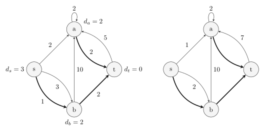
Run a single-source shortest path algorithm from the target vertex \(t\) on the reversed graph, record the shortest path length \(h(x)\) from each vertex \(x\) to \(t\), and record the first edge \(f_x\) taken on the shortest path from vertex \(x\); if there are multiple optimal choices, any one can be selected. All these edges \(f_x\) and their endpoints form a tree, and the simple path from any vertex \(x\) on the tree to the root \(t\) is a shortest path from \(x\) to \(t\). This is the shortest path tree \(T\).

After obtaining the shortest path tree \(T\), the additional cost incurred by each edge not in \(T\) can be calculated. For an edge \(e=(u,v)\notin T\) with weight \(w\), a new edge can be defined, still from \(u\) to \(v\), with cost \(\Delta(e)=w + h(v) - h(u)\). This article figuratively calls these edges with weight \(\Delta(e)\) sidetrack edges, and the weight \(\Delta(e)\) is called the sidetrack cost. If an edge's endpoints are not all in the shortest path tree \(T\), it does not affect the computation of the \(k\) shortest paths to vertex \(t\) and can be directly removed.

The left side of the figure below is the directed graph \(G\), and the right side is its corresponding shortest path tree \(T\) (thick edges) and the corresponding sidetrack edges (thin edges):

Let the set of edges traversed by a path from \(s\) to \(t\) be \(P\), and remove the intersection of \(P\) with \(T\) to obtain \(P'\). Then, arranging the edges in \(P'\) in order, any two consecutive edges \(e_1=(u_1,v_1)\) and \(e_2=(u_2,v_2)\) must satisfy

• Condition \((*)\): The starting point \(u_2\) of the latter is an ancestor (including itself) of the ending point \(v_1\) of the former in the shortest path tree \(T\).

This is because in the corresponding original path \(P\), several tree edges from \(T\) connect \(v_1\) and \(u_2\). Conversely, for an edge set \(P'\) satisfying condition \((*)\), there exists a unique path \(P\) in graph \(G\) corresponding to it. This is because the simple path from \(v_1\) to \(u_2\) on the shortest path tree \(T\) is unique. This shows that any path \(P\) in the original graph corresponds one-to-one with a sidetrack edge sequence \(P'\) satisfying condition \((*)\). Moreover, the length of path \(P\) equals the sum of the shortest path length \(h(s)\) and these sidetrack costs:

\[ h(s)+\sum_{e\in P'}\Delta(e). \]

This discussion indicates that the task of finding the \(k\) shortest paths transforms into the task of finding the \(k\)-th smallest cost sidetrack edge sequence \(P'\) satisfying condition \((*)\).

To handle condition \((*)\), instead of searching for ancestors in the shortest path tree each time during queries, it is better to directly propagate each vertex's sidetrack edge set down to its descendants in the shortest path tree. This is equivalent to constructing the following graph \(G'\):

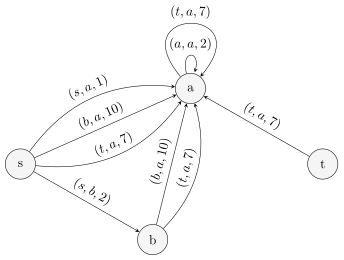
In this graph, condition \((*)\) transforms into requiring that the edges in \(P'\) are connected end to end, meaning \(P'\) is a path in graph \(G'\). The problem further transforms into finding the \(k\)-th smallest length path to any vertex starting from \(s\) in this graph. Compared to the original \(k\) shortest paths problem, it is no longer required that the path must end at the target vertex \(t\).

The transformed problem is easy to solve. Simply start from the starting vertex \(s\) and compute single-source shortest paths. Each time a vertex is extracted from the priority queue, it corresponds to finding a path in graph \(G'\), which in turn corresponds to a path to the target vertex \(t\) in graph \(G\).

Persistent Mergeable Heap Optimization

The algorithmic idea is now clear. However, a naive implementation of this algorithm is too inefficient. In graph \(G'\), the size of edges at a single vertex could be \(\Theta(m)\), so each time single-source shortest paths are computed, an edge set of size \(\Theta(m)\) may need to be pushed into the priority queue. Actually, it is unnecessary to push all edges into the priority queue: in many cases, among these edges pushed into the queue, only the shortest ones might be popped later. That is, the entire edge set at a single vertex can be treated as a single unit pushed into the priority queue, and only the shortest edge in the set needs to be quickly accessed each time.

This inspires us to use a min-heap to store the edge set at a single vertex. In the priority queue for single-source shortest paths, only these heaps need to be stored, and their cost is the shortest path cost corresponding to the heap's top element. Each time the front of the queue is popped, the top edge must also be popped from the heap at the front. Then, both the heap after popping its top must be pushed back into the priority queue, and the heap top corresponding to the sidetrack edge set at the endpoint of the popped top edge must be pushed into the priority queue.

Using heaps to store edge sets also solves the problem of propagating edge sets down the shortest path tree. Because propagating edge sets down is equivalent to merging the current vertex's edge set into its child vertices, the heap must also support merge operations; meanwhile, merging into child vertices must not destroy the edge set at the current vertex, so the heap must also support persistence. This is exactly a persistent mergeable heap.

Thus, the complete algorithm process is obtained:

1. Starting from the target vertex \(t\), run single-source shortest paths to obtain the shortest path tree.
2. For each vertex in the shortest path tree, construct its corresponding sidetrack edge set and store it in a persistent mergeable heap.
3. Along the edges of the shortest path tree, starting from the target vertex \(t\), merge each vertex's heap into its child vertices' heaps.
4. Starting from the starting vertex \(s\), push its heap into the priority queue.
5. Pop the heap at the front of the queue, record the answer, then push the heap after popping its top back into the priority queue, and push the heap at the endpoint of the popped top edge into the priority queue.

Persistent mergeable heaps are usually implemented using leftist heaps or randomized heaps. In this case, the last step can be further optimized. The internal structure of these heaps is a binary tree. After popping the heap top, originally the two child nodes would be merged, and the merged heap top would be pushed into the priority queue; however, in this algorithm, the merge operation can be skipped, and the two child nodes' corresponding heaps can be directly pushed into the priority queue separately. This saves the \(O(\log m)\) complexity of a single merge. Since each time the front heap is popped, at most three new heaps are pushed into the priority queue, the size of the priority queue is \(O(k)\). Thus, the time complexity of a single query is reduced to \(O(\log k)\). The total query complexity becomes \(O(k\log k)\).

Since constructing the shortest path tree and constructing the persistent mergeable heaps both have complexity \(O(m\log m)\), the total time complexity of the algorithm is \(O(m\log m+k\log k)\).

Implementation

Reference implementation for template problem Library Checker - K-Shortest Walk

// Submission: https://judge.yosupo.jp/submission/311623
#include <algorithm>
#include <iostream>
#include <queue>
#include <random>
#include <vector>

std::mt19937_64 rng(static_cast<std::mt19937_64::result_type>(time(nullptr)));

constexpr long long inf = 0x3f3f3f3f3f3f3f3f;

// Persistent Randomized Heap.
struct PersistentRandomizedHeap {
  static constexpr int N = 1e7;
  int id;
  std::vector<int> rt, lc, rc, to;
  std::vector<long long> va;

  int new_node(long long cost, int _to) {
    ++id;
    va[id] = cost;
    to[id] = _to;
    return id;
  }

  int copy_node(int x) {
    ++id;
    lc[id] = lc[x];
    rc[id] = rc[x];
    va[id] = va[x];
    to[id] = to[x];
    return id;
  }

  int meld(int x, int y, std::mt19937_64::result_type rand) {
    if (!x || !y) return x | y;
    if (va[x] > va[y]) std::swap(x, y);
    x = copy_node(x);
    if (rand & 1) std::swap(lc[x], rc[x]);
    rc[x] = meld(rc[x], y, rand >> 1);
    return x;
  }

  PersistentRandomizedHeap() : id(0), rt(N), lc(N), rc(N), to(N), va(N) {}

  void insert(int i, long long cost, int _to) {
    rt[i] = meld(rt[i], new_node(cost, _to), rng());
  }

  void merge(int i, int j) { rt[i] = meld(rt[i], rt[j], rng()); }

} heaps;

struct Edge {
  int u, v, c;

  Edge(int u, int v, int c) : u(u), v(v), c(c) {}
};

int n, m, s, t, k;
std::vector<std::vector<int>> gr, ig;
std::vector<Edge> edges;
std::priority_queue<std::pair<long long, int>,
                    std::vector<std::pair<long long, int>>, std::greater<>>
    pq;

std::vector<long long> dist_t;
std::vector<int> out;

// Calculate distances to the destination node t. (Dijkstra)
// Record the optimal outgoing edges which form the shortest path tree T.
void calc_distances_to_t() {
  dist_t.assign(n, inf);
  dist_t[t] = 0;
  out.assign(n, -1);
  pq.emplace(dist_t[t], t);
  while (!pq.empty()) {
    long long di = pq.top().first;
    int cur = pq.top().second;
    pq.pop();
    if (di > dist_t[cur]) continue;
    for (auto e : ig[cur]) {
      int nxt = edges[e].u;
      auto di_nxt = di + edges[e].c;
      if (di_nxt < dist_t[nxt]) {
        dist_t[nxt] = di_nxt;
        out[nxt] = e;
        pq.emplace(di_nxt, nxt);
      }
    }
  }
}

// Construct sidetracks and propagate them through tree T.
void build_sidetracks() {
  // Insert all valid sidetracks into heaps.
  for (int i = 0; i < m; ++i) {
    auto edge = edges[i];
    if (out[edge.u] != i && dist_t[edge.u] < inf && dist_t[edge.v] < inf) {
      heaps.insert(edge.u, edge.c + dist_t[edge.v] - dist_t[edge.u], edge.v);
    }
  }
  // Propagate sidetracks down the shortest path tree.
  std::queue<int> q;
  q.push(t);
  while (!q.empty()) {
    auto cur = q.front();
    q.pop();
    for (auto e : ig[cur]) {
      auto nxt = edges[e].u;
      if (out[nxt] == e) {
        heaps.merge(nxt, cur);
        q.push(nxt);
      }
    }
  }
}

std::vector<long long> ans;

// Insert a non-empty heap into the priority queue.
// Total cost is the heap top value adjusted by accumulated cost.
void insert(int x, long long cost) {
  if (x) pq.emplace(cost + heaps.va[x], x);
}

// Find the k shortest paths in the sidetrack graph. (Dijkstra)
// These correspond to the k shortest walks in the original graph.
void find_k_shortest_walks() {
  int cnt = 0;
  ans.assign(k, -1);
  if (dist_t[s] >= inf) return;
  ans[cnt++] = dist_t[s];
  insert(heaps.rt[s], dist_t[s]);
  while (!pq.empty() && cnt < k) {
    auto cost = pq.top().first;
    int cur = pq.top().second;
    pq.pop();
    ans[cnt++] = cost;
    insert(heaps.lc[cur], cost - heaps.va[cur]);
    insert(heaps.rc[cur], cost - heaps.va[cur]);
    insert(heaps.rt[heaps.to[cur]], cost);
  }
}

int main() {
  // Input.
  std::cin >> n >> m >> s >> t >> k;
  gr.resize(n);
  ig.resize(n);
  edges.reserve(m);
  for (int i = 0; i < m; ++i) {
    int u, v, c;
    std::cin >> u >> v >> c;
    edges.emplace_back(u, v, c);
    gr[u].push_back(i);
    ig[v].push_back(i);
  }
  // Calculate.
  calc_distances_to_t();
  build_sidetracks();
  find_k_shortest_walks();
  // Output.
  for (auto x : ans) std::cout << x << '\n';
  return 0;
}

Exercises

• 「SDOI2010」Magic Pig Academy

References and Notes

• [Tutorial] k shortest paths and Eppstein's algorithm by meooow - Codeforces

---

本页面最近更新：，更新历史
发现错误？想一起完善？ 在 GitHub 上编辑此页！
本页面贡献者：OI-wiki
本页面的全部内容在 CC BY-SA 4.0 和 SATA 协议之条款下提供，附加条款亦可能应用