Arbitrary-Precision Arithmetic

TL;DR: Template at the end...

Definition

Arbitrary-Precision Arithmetic, also known as bignum arithmetic, uses certain algorithmic structures to support operations on integers larger than those supported by the language's built-in integer types (numbers exceeding the language's native integer range).

Introduction

Arbitrary-precision arithmetic involves many small details and requires careful implementation.

So today, let's implement a simple calculator together.

Task

Input: An expression of the form a <op> b.

• a and b are non-negative decimal integers with length not exceeding \(1000\);
• <op> is a character (+, -, *, or /) representing the operation.
• There is a single space between the integer and the operator.

Output: The result of the operation.

• For +, -, and * operations, output one line representing the result;
• For the / operation, output two lines representing the quotient and remainder, respectively.
• It is guaranteed that all results are non-negative integers.

Storage

In typical implementations, arbitrary-precision numbers are represented as strings, where each character represents a decimal digit. Therefore, arbitrary-precision numerical computation can be seen as a special kind of string processing.

When reading a string, the most significant digit is at the beginning of the string (the position with a smaller index). However, by convention, the position with the smallest index stores the least significant digit of the number, meaning the string is stored in reverse. The reason for this is that the length of the number may change, but we want digits of the same place value to remain aligned (e.g., all ones digits at index [0], all tens digits at index [1], etc.). Additionally, addition, subtraction, and multiplication operations generally start from the ones digit (recall elementary school column arithmetic), which provides ample justification for "reverse storage".

We will adhere to this convention hereafter. Define a constant LEN = 1004 to represent the maximum length accommodated by the program.

Thus, it's straightforward to write the code for reading an arbitrary-precision number:

void clear(int a[]) {
  for (int i = 0; i < LEN; ++i) a[i] = 0;
}

void read(int a[]) {
  static char s[LEN + 1];
  scanf("%s", s);

  clear(a);

  int len = strlen(s);
  // As mentioned above, reverse
  for (int i = 0; i < len; ++i) a[len - i - 1] = s[i] - '0';
  // s[i] - '0' is the digit represented by s[i]
  // Some may be more accustomed to understanding it as ord(s[i]) - ord('0')
}

Output is also in reverse order of storage. Since we don't want to output leading zeros, we start from the most significant digit and search downward for the first non-zero digit, then output from there. The termination condition is i >= 1 instead of i >= 0 because we still want to output a single character 0 when the entire number equals \(0\).

void print(int a[]) {
  int i;
  for (i = LEN - 1; i >= 1; --i)
    if (a[i] != 0) break;
  for (; i >= 0; --i) putchar(a[i] + '0');
  putchar('\n');
}

Putting it together, we have a complete repeater program.

copycat.cpp

#include <cstdio>
#include <cstring>

constexpr int LEN = 1004;

int a[LEN];

void clear(int a[]) {
  for (int i = 0; i < LEN; ++i) a[i] = 0;
}

void read(int a[]) {
  static char s[LEN + 1];
  scanf("%s", s);

  clear(a);

  int len = strlen(s);
  for (int i = 0; i < len; ++i) a[len - i - 1] = s[i] - '0';
}

void print(int a[]) {
  int i;
  for (i = LEN - 1; i >= 1; --i)
    if (a[i] != 0) break;
  for (; i >= 0; --i) putchar(a[i] + '0');
  putchar('\n');
}

int main() {
  read(a);
  print(a);

  return 0;
}

Arithmetic Operations

The difficulty of the four basic operations varies. The simplest are arbitrary-precision addition and subtraction, followed by arbitrary-precision–single-precision (ordinary int) multiplication and arbitrary-precision–arbitrary-precision multiplication, with arbitrary-precision–arbitrary-precision division being the most complex.

We will implement all required functions in this order.

Addition

Arbitrary-precision addition is essentially column addition.

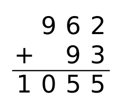
That is, starting from the least significant digit, add the digits at corresponding positions of the two addends and determine whether the sum reaches or exceeds \(10\). If it does, handle the carry: increment the result at the next higher position by \(1\), and reduce the current digit's result by \(10\).

void add(int a[], int b[], int c[]) {
  clear(c);

  // In arbitrary-precision implementations, the maximum array length LEN is usually set slightly larger than the possible input
  // Then, the last few iterations are omitted, which saves a lot of boundary case handling
  // Since the actual input won't exceed 1000 digits, iterating to LEN - 1 = 1003 is sufficient here
  for (int i = 0; i < LEN - 1; ++i) {
    // Add the digits at the corresponding positions
    c[i] += a[i] + b[i];
    if (c[i] >= 10) {
      // Carry
      c[i + 1] += 1;
      c[i] -= 10;
    }
  }
}

Combining this with the previous part yields an addition calculator.

adder.cpp

#include <cstdio>
#include <cstring>

constexpr int LEN = 1004;

int a[LEN], b[LEN], c[LEN];

void clear(int a[]) {
  for (int i = 0; i < LEN; ++i) a[i] = 0;
}

void read(int a[]) {
  static char s[LEN + 1];
  scanf("%s", s);

  clear(a);

  int len = strlen(s);
  for (int i = 0; i < len; ++i) a[len - i - 1] = s[i] - '0';
}

void print(int a[]) {
  int i;
  for (i = LEN - 1; i >= 1; --i)
    if (a[i] != 0) break;
  for (; i >= 0; --i) putchar(a[i] + '0');
  putchar('\n');
}

void add(int a[], int b[], int c[]) {
  clear(c);

  for (int i = 0; i < LEN - 1; ++i) {
    c[i] += a[i] + b[i];
    if (c[i] >= 10) {
      c[i + 1] += 1;
      c[i] -= 10;
    }
  }
}

int main() {
  read(a);
  read(b);

  add(a, b, c);
  print(c);

  return 0;
}

Subtraction

Arbitrary-precision subtraction is essentially column subtraction.

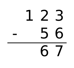
Subtract digit by digit starting from the ones place, borrowing \(1\) from the next higher digit when a negative result occurs. The overall approach is exactly the same as addition.

void sub(int a[], int b[], int c[]) {
  clear(c);

  for (int i = 0; i < LEN - 1; ++i) {
    // Subtract digit by digit
    c[i] += a[i] - b[i];
    if (c[i] < 0) {
      // Borrow
      c[i + 1] -= 1;
      c[i] += 10;
    }
  }
}

Replacing add() with sub() in the previous program yields a subtraction calculator.

subtractor.cpp

#include <cstdio>
#include <cstring>

constexpr int LEN = 1004;

int a[LEN], b[LEN], c[LEN];

void clear(int a[]) {
  for (int i = 0; i < LEN; ++i) a[i] = 0;
}

void read(int a[]) {
  static char s[LEN + 1];
  scanf("%s", s);

  clear(a);

  int len = strlen(s);
  for (int i = 0; i < len; ++i) a[len - i - 1] = s[i] - '0';
}

void print(int a[]) {
  int i;
  for (i = LEN - 1; i >= 1; --i)
    if (a[i] != 0) break;
  for (; i >= 0; --i) putchar(a[i] + '0');
  putchar('\n');
}

void sub(int a[], int b[], int c[]) {
  clear(c);

  for (int i = 0; i < LEN - 1; ++i) {
    c[i] += a[i] - b[i];
    if (c[i] < 0) {
      c[i + 1] -= 1;
      c[i] += 10;
    }
  }
}

int main() {
  read(a);
  read(b);

  sub(a, b, c);
  print(c);

  return 0;
}

Try it: input 1 2—output /9999999, huh, why is this OI Wiki giving me fake code...

Actually, the above code only handles the case where the minuend \(a\) is greater than or equal to the subtrahend \(b\). Handling the case where the minuend is smaller than the subtrahend, i.e., \(a<b\), is simple.

\(a-b=-(b-a)\)

To compute \(b-a\), since \(b>a\), we can call the sub function from the above code as sub(b,a,c). To obtain \(a-b\), simply prepend a negative sign to the result.

Multiplication

Arbitrary-Precision–Single-Precision

Arbitrary-precision multiplication, that is, column... wait a minute!

First, consider a simple case: one of the multipliers is an ordinary int. Is there a simple way to handle this?

An intuitive approach is to directly multiply each digit of \(a\) by \(b\). Numerically, this method is correct, but it does not conform to decimal representation, so it needs to be reorganized into a normal form.

The reorganization method also processes carries digit by digit from the least significant digit upward. However, the carry here can be very large, even much larger than \(9\), because each digit after multiplication can reach the magnitude of \(9b\). Therefore, the carry can no longer be simply handled by a \(-10\) operation; instead, it must be computed using the quotient and remainder of division by \(10\). See the code comments for details, or refer to the diagram below illustrating the process of multiplying the arbitrary-precision number \(1337\) by the single-precision number \(42\).

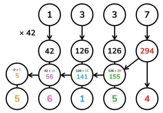
Of course, for this reason, this method requires special attention to the range of the multiplier \(b\). If it is on the same order of magnitude as \(10^9\) (or the upper bound of the corresponding integer type), then arbitrary-precision–single-precision multiplication should be used with caution.

void mul_short(int a[], int b, int c[]) {
  clear(c);

  for (int i = 0; i < LEN - 1; ++i) {
    // Directly multiply the i-th digit of a by the multiplier and add to the result
    c[i] += a[i] * b;

    if (c[i] >= 10) {
      // Handle carry
      // c[i] / 10, the quotient of division, becomes the increment for the carry
      c[i + 1] += c[i] / 10;
      // And c[i] % 10, the remainder of division, becomes the value left at the current digit
      c[i] %= 10;
    }
  }
}

Arbitrary-Precision–Arbitrary-Precision

If both multipliers are arbitrary-precision, then column multiplication can shine again.

Recall each step of column multiplication: it actually computes the sum of several terms \(a \times b_i \times 10^i\). For example, to compute \(1337 \times 42\), we compute \(1337 \times 2 \times 10^0 + 1337 \times 4 \times 10^1\).

Thus, we can decompose \(b\) into all its digits, each of which is a single-precision number, multiply them separately by \(a\), shift them left to their respective positions, and then add them to get the answer. Of course, carries must also be handled uniformly at the end, as in the previous example.

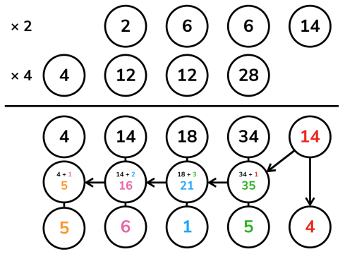
Note that this process is not exactly the same as column multiplication. Our algorithm does not carry during each multiplication step; instead, it retains all results in their corresponding positions and processes carries uniformly at the end, but this does not affect the result.

void mul(int a[], int b[], int c[]) {
  clear(c);

  for (int i = 0; i < LEN - 1; ++i) {
    // Here we directly compute the i-th digit (from least significant) of the result and handle carries simultaneously
    // The i-th iteration adds to c[i] the sum of all products a[p] * b[q] where p + q = i
    // This achieves the same effect as performing the operations in the diagram above and summing at the end, but is a more concise implementation
    for (int j = 0; j <= i; ++j) c[i] += a[j] * b[i - j];

    if (c[i] >= 10) {
      c[i + 1] += c[i] / 10;
      c[i] %= 10;
    }
  }
}

Division

One implementation of arbitrary-precision division is long division.

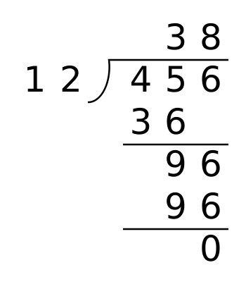
Long division can actually be seen as a process of successive subtractions. For example, the calculation of the tens digit of the quotient in the diagram above can be understood as: after subtracting \(12\) from \(45\) three times, the result becomes less than \(12\) and cannot be subtracted further, so this digit is \(3\).

To reduce redundant computations, we first obtain the length \(l_a\) of the dividend and the length \(l_b\) of the divisor, and start computing the quotient from index \(l_a - l_b\), from the most significant digit to the least significant digit. This aligns the highest digit of the first multiplication with the highest digit of the dividend, just like in manual calculation.

The reference implementation provides a function greater_eq() to determine whether the dividend, with its lowest digit at index last_dg, can subtract the divisor while remaining non-negative. Then, for each digit of the quotient, it repeatedly calls greater_eq(), and when it holds, uses arbitrary-precision subtraction to subtract the divisor from the remainder, simulating the long division process.

// Whether the dividend a, with its lowest digit at index last_dg, can subtract divisor b and remain non-negative
// len is the length of divisor b, to avoid repeated computation
bool greater_eq(int a[], int b[], int last_dg, int len) {
  // The remaining part of the dividend might be longer than the divisor; in this case, it can be at most one digit longer, so this check suffices
  if (a[last_dg + len] != 0) return true;
  // Compare digit by digit from most significant to least significant
  for (int i = len - 1; i >= 0; --i) {
    if (a[last_dg + i] > b[i]) return true;
    if (a[last_dg + i] < b[i]) return false;
  }
  // Equality is also acceptable
  return true;
}

void div(int a[], int b[], int c[], int d[]) {
  clear(c);
  clear(d);

  int la, lb;
  for (la = LEN - 1; la > 0; --la)
    if (a[la - 1] != 0) break;
  for (lb = LEN - 1; lb > 0; --lb)
    if (b[lb - 1] != 0) break;
  if (lb == 0) {  // Divisor cannot be zero
    puts("> <");
    return;
  }

  // c is the quotient
  // d is the remaining part of the dividend, which naturally becomes the remainder after the algorithm ends
  for (int i = 0; i < la; ++i) d[i] = a[i];
  for (int i = la - lb; i >= 0; --i) {
    // Compute the i-th digit of the quotient
    while (greater_eq(d, b, i, lb)) {
      // If subtraction is possible, subtract
      // This segment is an arbitrary-precision subtraction
      for (int j = 0; j < lb; ++j) {
        d[i + j] -= b[j];
        if (d[i + j] < 0) {
          d[i + j + 1] -= 1;
          d[i + j] += 10;
        }
      }
      // Increment this digit of the quotient by 1
      c[i] += 1;
      // Return to the beginning of the loop to recheck
    }
  }
}

Introductory Section Complete!

Combining the implementations of the four arithmetic operations described above completes the calculator program mentioned at the beginning.

calculator.cpp

#include <cstdio>
#include <cstring>

constexpr int LEN = 1004;

int a[LEN], b[LEN], c[LEN], d[LEN];

void clear(int a[]) {
  for (int i = 0; i < LEN; ++i) a[i] = 0;
}

void read(int a[]) {
  static char s[LEN + 1];
  scanf("%s", s);

  clear(a);

  int len = strlen(s);
  for (int i = 0; i < len; ++i) a[len - i - 1] = s[i] - '0';
}

void print(int a[]) {
  int i;
  for (i = LEN - 1; i >= 1; --i)
    if (a[i] != 0) break;
  for (; i >= 0; --i) putchar(a[i] + '0');
  putchar('\n');
}

void add(int a[], int b[], int c[]) {
  clear(c);

  for (int i = 0; i < LEN - 1; ++i) {
    c[i] += a[i] + b[i];
    if (c[i] >= 10) {
      c[i + 1] += 1;
      c[i] -= 10;
    }
  }
}

void sub(int a[], int b[], int c[]) {
  clear(c);

  for (int i = 0; i < LEN - 1; ++i) {
    c[i] += a[i] - b[i];
    if (c[i] < 0) {
      c[i + 1] -= 1;
      c[i] += 10;
    }
  }
}

void mul(int a[], int b[], int c[]) {
  clear(c);

  for (int i = 0; i < LEN - 1; ++i) {
    for (int j = 0; j <= i; ++j) c[i] += a[j] * b[i - j];

    if (c[i] >= 10) {
      c[i + 1] += c[i] / 10;
      c[i] %= 10;
    }
  }
}

bool greater_eq(int a[], int b[], int last_dg, int len) {
  if (a[last_dg + len] != 0) return true;
  for (int i = len - 1; i >= 0; --i) {
    if (a[last_dg + i] > b[i]) return true;
    if (a[last_dg + i] < b[i]) return false;
  }
  return true;
}

void div(int a[], int b[], int c[], int d[]) {
  clear(c);
  clear(d);

  int la, lb;
  for (la = LEN - 1; la > 0; --la)
    if (a[la - 1] != 0) break;
  for (lb = LEN - 1; lb > 0; --lb)
    if (b[lb - 1] != 0) break;
  if (lb == 0) {
    puts("> <");
    return;
  }

  for (int i = 0; i < la; ++i) d[i] = a[i];
  for (int i = la - lb; i >= 0; --i) {
    while (greater_eq(d, b, i, lb)) {
      for (int j = 0; j < lb; ++j) {
        d[i + j] -= b[j];
        if (d[i + j] < 0) {
          d[i + j + 1] -= 1;
          d[i + j] += 10;
        }
      }
      c[i] += 1;
    }
  }
}

int main() {
  read(a);

  char op[4];
  scanf("%s", op);

  read(b);

  switch (op[0]) {
    case '+':
      add(a, b, c);
      print(c);
      break;
    case '-':
      sub(a, b, c);
      print(c);
      break;
    case '*':
      mul(a, b, c);
      print(c);
      break;
    case '/':
      div(a, b, c, d);
      print(c);
      print(d);
      break;
    default:
      puts("> <");
  }

  return 0;
}

Digit-Packing Arbitrary-Precision Arithmetic

Introduction

In general arbitrary-precision addition, subtraction, and multiplication, we split the numbers involved into individual digits for computation.

For example, when computing \(8192\times 42\), if we follow the arbitrary-precision–arbitrary-precision multiplication method, we are actually computing \((8000+100+90+2)\times(40+2)\).

When the number of digits is large, the number of split digits also increases, and the efficiency of arbitrary-precision operations decreases.

Is there a way to optimize this?

Note that the method of splitting digits does not affect the final result, so we can merge several digits together.

Process

Using the same example, if we split every two digits into one number, we can split it into \((8100+92)\times 42\).

Such splitting does not affect the final result, but because the number of split digits is reduced, computational efficiency improves.

Understanding this process from the perspective of numeral systems, we perform operations in a larger base (splitting every two digits above can be considered as operating in base \(100\)) to reduce the number of digits involved in operations, thereby improving efficiency.

This is the idea behind digit-packing arbitrary-precision arithmetic.

Below we provide a reference implementation of digit-packing arbitrary-precision addition to further illustrate its implementation:

Reference Implementation of Digit-Packing Arbitrary-Precision Addition

// Here, arrays a, b, c are numbers in base p
// The final output requires converting the numbers to decimal
void add(int a[], int b[], int c[]) {
  clear(c);

  for (int i = 0; i < LEN - 1; ++i) {
    c[i] += a[i] + b[i];
    if (c[i] >= p) {  // In ordinary arbitrary-precision arithmetic, p=10
      c[i + 1] += 1;
      c[i] -= p;
    }
  }
}

Efficient Long Division with Digit-Packing

When using digit-packing, if trial division is still performed using the method described earlier, the number of trial divisions will be very high, resulting in a large constant factor. For example, in base 10,000, each digit requires an average of 5000 trial divisions, which is an unacceptable constant. Therefore, we need a more efficient trial division method.

We can use double as an intermediary. Suppose the dividend has 4 digits: \(a_4,a_3,a_2,a_1\), and the divisor has 3 digits: \(b_3,b_2,b_1\). Then we only need to trial one digit of the quotient: using base \(base\), estimate the quotient with the expression \(\dfrac{a_4 base + a_3}{b_3 + b_2 base^{-1} + (b_1+1)base^{-2}}\). For multiple digits, it's the single-digit method plus a loop. Since the divisor uses 3-digit precision to estimate the quotient, it ensures that the estimated quotient \(q'\) and the actual quotient \(q\) satisfy \(q-1 \le q' \le q\), so each digit requires at most two trial divisions in the worst case. However, this requires that \(base^3\) fits within the effective precision of double, i.e., \(base^3 < 2^{53}\), so when using this method, it is recommended not to exceed base 32768; otherwise, errors due to insufficient precision can easily lead to mistakes.

Additionally, since the estimated quotient is always less than or equal to the actual quotient, there is room for further optimization. In most cases, each digit is estimated only once. When estimating the next digit, the estimated quotient might be greater than or equal to the base due to errors from the previous digit, but that's fine as long as we perform a unified carry at the end. For example, suppose the base is 10, and we compute \(395081/9876\). The trial division steps are as follows:

1. First trial division yields \(3950/988=3\), so \(395081-(9876 \times 3 \times 10^1) = 98801\). An error occurs here, but we ignore it and continue.
2. Continue trial division on the remainder 98801: \(9880/988=10\), so \(98801-(9876 \times 10 \times 10^0) = 41\), which is the final remainder.
3. Sum the results of the trial division process and handle carries: \(3 \times 10^1 + 10 \times 10^0 = 40\), which is the exact quotient.

Although the method seems simple, implementation is tricky. Therefore, we provide a reference implementation that has been verified multiple times to be correct. Important details are also noted in the comments.

Reference Implementation of Efficient Long Division with Digit-Packing

// Full template and implementation: https://baobaobear.github.io/post/20210228-bigint1/
// Subtract the result of multiplying b by mul and shifting left by offset, for division
BigIntSimple &sub_mul(const BigIntSimple &b, int mul, int offset) {
  if (mul == 0) return *this;
  int borrow = 0;
  // Unlike subtraction, borrow can be very large, so the subtraction approach cannot be used
  for (size_t i = 0; i < b.v.size(); ++i) {
    borrow += v[i + offset] - b.v[i] * mul - BIGINT_BASE + 1;
    v[i + offset] = borrow % BIGINT_BASE + BIGINT_BASE - 1;
    borrow /= BIGINT_BASE;
  }
  // Continue processing if there's still a borrow
  for (size_t i = b.v.size(); borrow; ++i) {
    borrow += v[i + offset] - BIGINT_BASE + 1;
    v[i + offset] = borrow % BIGINT_BASE + BIGINT_BASE - 1;
    borrow /= BIGINT_BASE;
  }
  return *this;
}

BigIntSimple div_mod(const BigIntSimple &b, BigIntSimple &r) const {
  BigIntSimple d;
  r = *this;
  if (absless(b)) return d;
  d.v.resize(v.size() - b.v.size() + 1);
  // Precompute the reciprocal of the divisor's top three digits + 1. If the top three digits are a3,a2,a1
  // then db is the reciprocal of a3+a2/base+(a1+1)/base^2. Finally, use multiplication to estimate each digit of the quotient.
  // This method works within int32 when BIGINT_BASE<=32768.
  // Even with int64, it only works when BIGINT_BASE<=131072 (due to double precision limitations).
  // It ensures that the estimated result q' and the actual result q satisfy q'<=q<=q'+1.
  // So each digit requires an average of only one trial division, and carries can be handled uniformly later.
  // For larger bases, other trial division schemes must be used.
  double t = (b.get((unsigned)b.v.size() - 2) +
              (b.get((unsigned)b.v.size() - 3) + 1.0) / BIGINT_BASE);
  double db = 1.0 / (b.v.back() + t / BIGINT_BASE);
  for (size_t i = v.size() - 1, j = d.v.size() - 1; j <= v.size();) {
    int rm = r.get(i + 1) * BIGINT_BASE + r.get(i);
    int m = std::max((int)(db * rm), r.get(i + 1));
    r.sub_mul(b, m, j);
    d.v[j] += m;
    if (!r.get(i + 1))  // Check if the highest digit is already 0 to avoid edge cases
      --i, --j;
  }
  r.trim();
  // Adjust the units digit of the result
  int carry = 0;
  while (!r.absless(b)) {
    r.subtract(b);
    ++carry;
  }
  // Adjust carries for each digit
  for (size_t i = 0; i < d.v.size(); ++i) {
    carry += d.v[i];
    d.v[i] = carry % BIGINT_BASE;
    carry /= BIGINT_BASE;
  }
  d.trim();
  d.sign = sign * b.sign;
  return d;
}

BigIntSimple operator/(const BigIntSimple &b) const {
  BigIntSimple r;
  return div_mod(b, r);
}

BigIntSimple operator%(const BigIntSimple &b) const {
  BigIntSimple r;
  div_mod(b, r);
  return r;
}

Karatsuba Multiplication

Let the number of digits of an arbitrary-precision number be \(n\). Then arbitrary-precision–arbitrary-precision column multiplication takes \(O(n^2)\) time. This section introduces a more time-efficient algorithm proposed by the former Soviet (Russian) mathematician Anatoly Karatsuba, which is a divide-and-conquer algorithm.

Consider two decimal integers \(x\) and \(y\), each containing \(n\) digits (leading zeros allowed). Choose any \(0 < m < n\), and let

\[ \begin{aligned} x &= x_1 \cdot 10^m + x_0, \\ y &= y_1 \cdot 10^m + y_0, \\ x \cdot y &= z_2 \cdot 10^{2m} + z_1 \cdot 10^m + z_0, \end{aligned} \]

where \(x_0, y_0, z_0, z_1 < 10^m\). Then

\[ \begin{aligned} z_2 &= x_1 \cdot y_1, \\ z_1 &= x_1 \cdot y_0 + x_0 \cdot y_1, \\ z_0 &= x_0 \cdot y_0. \end{aligned} \]

Observe that

\[ z_1 = (x_1 + x_0) \cdot (y_1 + y_0) - z_2 - z_0, \]

so to compute \(z_1\), we only need to compute \((x_1 + x_0) \cdot (y_1 + y_0)\) and then subtract \(z_0\) and \(z_2\).

The above equation is actually the core of Karatsuba's algorithm. It transforms a multiplication problem of length \(n\) into three smaller subproblems. If we let \(m = \left\lceil \dfrac n 2 \right\rceil\), and denote the time taken by Karatsuba's algorithm to multiply two \(n\)-digit integers as \(T(n)\), then \(T(n) = 3 \cdot T \left(\left\lceil \dfrac n 2 \right\rceil\right) + O(n)\). By the master theorem, \(T(n) = \Theta(n^{\log_2 3}) \approx \Theta(n^{1.585})\).

The entire process can be implemented recursively. For clarity, the code below implements polynomial multiplication via Karatsuba's algorithm and finally handles all carry issues.

karatsuba_mulc.cpp

int *karatsuba_polymul(int n, int *a, int *b) {
  if (n <= 32) {
    // For small sizes, compute directly to avoid efficiency loss from further recursion
    int *r = new int[n * 2 + 1]();
    for (int i = 0; i <= n; ++i)
      for (int j = 0; j <= n; ++j) r[i + j] += a[i] * b[j];
    return r;
  }

  int m = n / 2 + 1;
  int *r = new int[m * 4 + 1]();
  int *z0, *z1, *z2;

  z0 = karatsuba_polymul(m - 1, a, b);
  z2 = karatsuba_polymul(n - m, a + m, b + m);

  // Compute z1
  // Temporarily modify, then restore after computation
  for (int i = 0; i + m <= n; ++i) a[i] += a[i + m];
  for (int i = 0; i + m <= n; ++i) b[i] += b[i + m];
  z1 = karatsuba_polymul(m - 1, a, b);
  for (int i = 0; i + m <= n; ++i) a[i] -= a[i + m];
  for (int i = 0; i + m <= n; ++i) b[i] -= b[i + m];
  for (int i = 0; i <= (m - 1) * 2; ++i) z1[i] -= z0[i];
  for (int i = 0; i <= (n - m) * 2; ++i) z1[i] -= z2[i];

  // Combine results from z0, z1, z2
  for (int i = 0; i <= (m - 1) * 2; ++i) r[i] += z0[i];
  for (int i = 0; i <= (m - 1) * 2; ++i) r[i + m] += z1[i];
  for (int i = 0; i <= (n - m) * 2; ++i) r[i + m * 2] += z2[i];

  delete[] z0;
  delete[] z1;
  delete[] z2;
  return r;
}

void karatsuba_mul(int a[], int b[], int c[]) {
  int *r = karatsuba_polymul(LEN - 1, a, b);
  memcpy(c, r, sizeof(int) * LEN);
  for (int i = 0; i < LEN - 1; ++i)
    if (c[i] >= 10) {
      c[i + 1] += c[i] / 10;
      c[i] %= 10;
    }
  delete[] r;
}

About new and delete

See Memory Pool.

However, such an implementation has a problem: in base \(b\), each coefficient of the polynomial can reach the magnitude of \(n \cdot b^2\), which may cause integer overflow in digit-packing arbitrary-precision implementations. If carries are handled during polynomial multiplication, then \(x_1 + x_0\) and \(y_1 + y_0\) can reach \(2 \cdot b^m\), adding an extra digit (if using \(x_1 - x_0\), negative numbers must be handled specially). Therefore, the implementation method should be chosen based on the actual application scenario.

Efficient Large Integer Multiplication Based on Polynomials

If the data scale reaches \(10^{10^5}\) or larger, ordinary arbitrary-precision multiplication may time out. This section introduces a method to optimize such multiplication using polynomials.

For an \(n\)-digit decimal integer \(a\), it can be viewed as a polynomial \(A=a_{0} 10^0+a_{1} 10^1+\cdots+a_{n-1} 10^{n-1}\) where each coefficient is an integer not exceeding \(10\). Thus, we transform integer multiplication into polynomial multiplication.

Ordinary polynomial multiplication still takes \(O(n^2)\) time, but it can be optimized using algorithms from the polynomial section, such as Fast Fourier Transform (FFT) and Number Theoretic Transform (NTT). The optimized time complexity is \(O(n\log n)\).

Encapsulated Classes

Here is an encapsulated arbitrary-precision integer class, and here is an ultra-minimal implementation class supporting dynamic length and four arithmetic operations.

Here is another template

constexpr int MAXN = 9999;
// MAXN is the largest digit in one position
constexpr int MAXSIZE = 10024;
// MAXSIZE is the number of digits
constexpr int DLEN = 4;

// DLEN records how many digits are packed
struct Big {
  int a[MAXSIZE], len;
  bool flag;  // Marks the sign '-'

  Big() {
    len = 1;
    memset(a, 0, sizeof a);
    flag = false;
  }

  Big(const int);
  Big(const char*);
  Big(const Big&);
  Big& operator=(const Big&);
  Big operator+(const Big&) const;
  Big operator-(const Big&) const;
  Big operator*(const Big&) const;
  Big operator/(const int&) const;
  // TODO: Big / Big;
  Big operator^(const int&) const;
  // TODO: Big ^ Big;

  // TODO: Big bitwise operations;

  int operator%(const int&) const;
  // TODO: Big ^ Big;
  bool operator<(const Big&) const;
  bool operator<(const int& t) const;
  void print() const;
};

Big::Big(const int b) {
  int c, d = b;
  len = 0;
  // memset(a,0,sizeof a);
  CLR(a);
  while (d > MAXN) {
    c = d - (d / (MAXN + 1) * (MAXN + 1));
    d = d / (MAXN + 1);
    a[len++] = c;
  }
  a[len++] = d;
}

Big::Big(const char* s) {
  int t, k, index, l;
  CLR(a);
  l = strlen(s);
  len = l / DLEN;
  if (l % DLEN) ++len;
  index = 0;
  for (int i = l - 1; i >= 0; i -= DLEN) {
    t = 0;
    k = i - DLEN + 1;
    if (k < 0) k = 0;
    g(j, k, i) t = t * 10 + s[j] - '0';
    a[index++] = t;
  }
}

Big::Big(const Big& T) : len(T.len) {
  CLR(a);
  f(i, 0, len) a[i] = T.a[i];
  // TODO: Overload here?
}

Big& Big::operator=(const Big& T) {
  CLR(a);
  len = T.len;
  f(i, 0, len) a[i] = T.a[i];
  return *this;
}

Big Big::operator+(const Big& T) const {
  Big t(*this);
  int big = len;
  if (T.len > len) big = T.len;
  f(i, 0, big) {
    t.a[i] += T.a[i];
    if (t.a[i] > MAXN) {
      ++t.a[i + 1];
      t.a[i] -= MAXN + 1;
    }
  }
  if (t.a[big])
    t.len = big + 1;
  else
    t.len = big;
  return t;
}

Big Big::operator-(const Big& T) const {
  int big;
  bool ctf;
  Big t1, t2;
  if (*this < T) {
    t1 = T;
    t2 = *this;
    ctf = true;
  } else {
    t1 = *this;
    t2 = T;
    ctf = false;
  }
  big = t1.len;
  int j = 0;
  f(i, 0, big) {
    if (t1.a[i] < t2.a[i]) {
      j = i + 1;
      while (t1.a[j] == 0) ++j;
      --t1.a[j--];
      // WTF?
      while (j > i) t1.a[j--] += MAXN;
      t1.a[i] += MAXN + 1 - t2.a[i];
    } else
      t1.a[i] -= t2.a[i];
  }
  t1.len = big;
  while (t1.len > 1 && t1.a[t1.len - 1] == 0) {
    --t1.len;
    --big;
  }
  if (ctf) t1.a[big - 1] = -t1.a[big - 1];
  return t1;
}

Big Big::operator*(const Big& T) const {
  Big res;
  int up;
  int te, tee;
  f(i, 0, len) {
    up = 0;
    f(j, 0, T.len) {
      te = a[i] * T.a[j] + res.a[i + j] + up;
      if (te > MAXN) {
        tee = te - te / (MAXN + 1) * (MAXN + 1);
        up = te / (MAXN + 1);
        res.a[i + j] = tee;
      } else {
        up = 0;
        res.a[i + j] = te;
      }
    }
    if (up) res.a[i + T.len] = up;
  }
  res.len = len + T.len;
  while (res.len > 1 && res.a[res.len - 1] == 0) --res.len;
  return res;
}

Big Big::operator/(const int& b) const {
  Big res;
  int down = 0;
  gd(i, len - 1, 0) {
    res.a[i] = (a[i] + down * (MAXN + 1)) / b;
    down = a[i] + down * (MAXN + 1) - res.a[i] * b;
  }
  res.len = len;
  while (res.len > 1 && res.a[res.len - 1] == 0) --res.len;
  return res;
}

int Big::operator%(const int& b) const {
  int d = 0;
  gd(i, len - 1, 0) d = (d * (MAXN + 1) % b + a[i]) % b;
  return d;
}

Big Big::operator^(const int& n) const {
  Big t(n), res(1);
  int y = n;
  while (y) {
    if (y & 1) res = res * t;
    t = t * t;
    y >>= 1;
  }
  return res;
}

bool Big::operator<(const Big& T) const {
  int ln;
  if (len < T.len) return true;
  if (len == T.len) {
    ln = len - 1;
    while (ln >= 0 && a[ln] == T.a[ln]) --ln;
    if (ln >= 0 && a[ln] < T.a[ln]) return true;
    return false;
  }
  return false;
}

bool Big::operator<(const int& t) const {
  Big tee(t);
  return *this < tee;
}

void Big::print() const {
  printf("%d", a[len - 1]);
  gd(i, len - 2, 0) { printf("%04d", a[i]); }
}

void print(const Big& s) {
  int len = s.len;
  printf("%d", s.a[len - 1]);
  gd(i, len - 2, 0) { printf("%04d", s.a[i]); }
}

char s[100024];

Exercises

• NOIP 2012 King's Game
• SPOJ - Fast Multiplication
• SPOJ - GCD2
• UVa - Division
• UVa - Fibonacci Freeze
• Codeforces - Notepad

References and Links

1. Karatsuba algorithm - Wikipedia

---

本页面最近更新：，更新历史
发现错误？想一起完善？ 在 GitHub 上编辑此页！
本页面贡献者：OI-wiki
本页面的全部内容在 CC BY-SA 4.0 和 SATA 协议之条款下提供，附加条款亦可能应用