Tree Divide and Conquer
Centroid Decomposition
Centroid decomposition is suitable for handling large-scale tree path information problems.
Example 1 Luogu P3806【Template】Centroid Decomposition 1
Given a tree with \(n\) vertices and edge weights, answer \(m\) queries. For each query, given \(k\), determine whether there exists a pair of vertices with distance exactly \(k\) on the tree.
\(n\le 10000,m\le 100,k\le 10000000\)
We first arbitrarily choose a node as the root \(\mathit{rt}\). All paths entirely within its subtree can be divided into two types: those passing through the current root node and those not passing through the current root node. For paths passing through the current root node, they can be further divided into two types: those with the root node as one endpoint, and those where neither endpoint is the root node. The latter can be obtained by merging two chains of the former type. Therefore, for the enumerated root node \(rt\), we first compute the contribution to the answer from paths within its subtree that pass through this node, then recursively solve for paths not passing through this node in its subtrees.
In this problem, for paths passing through the root node \(\mathit{rt}\), we first enumerate all its child nodes \(\mathit{ch}\), and compute the distances from all nodes in the \(\mathit{ch}\) subtree to \(\mathit{rt}\) with \(\mathit{ch}\) as the root. Let \(\mathit{dist}_i\) denote the distance from node \(i\) to the current root \(rt\), and \(\mathit{tf}_{d}\) indicate whether there exists a node \(v\) in previously processed subtrees such that \(\mathit{dist}_v=d\). If a query \(k\) satisfies \(tf_{k-\mathit{dist}_i}=true\), then there exists a path of length \(k\). After computing whether the edges connected in the \(\mathit{ch}\) subtree can form an answer, we add these new distances to the \(\mathit{tf}\) array.
Note that when clearing the \(\mathit{tf}\) array, we cannot simply use memset. Instead, we should add the previously used \(\mathit{tf}\) positions to a queue and clear them one by one. This ensures the time complexity.
During centroid decomposition, each node is processed once per level across all recursive calls in that level. Assuming there are \(h\) recursive levels in total, the overall time complexity is \(O(hn)\).
If we always select the centroid of the subtree as the root node, we can guarantee the minimum number of recursive levels, resulting in a time complexity of \(O(n\log n)\). Therefore, centroid decomposition is also commonly known as centroid decomposition in international competitive programming circles.
Please note that after reselecting the root node, it is essential to recalculate the subtree sizes. Otherwise, even a seemingly minor change may lead to incorrect time complexity or correctness issues.
Reference Code
1 2 3 4 5 6 7 8 9 10 11 12 13 14 15 16 17 18 19 20 21 22 23 24 25 26 27 28 29 30 31 32 33 34 35 36 37 38 39 40 41 42 43 44 45 46 47 48 49 50 51 52 53 54 55 56 57 58 59 60 61 62 63 64 65 66 67 68 69 70 71 | |
Example 2 Luogu P4178 Tree
Given a weighted tree with \(n\) vertices and an integer \(k\), count the number of vertex pairs whose distance on the tree is less than or equal to \(k\).
\(n\le 40000,k\le 20000,w_i\le 1000\)
Since here we query the number of vertex pairs with distances in \([0,k]\), we use a segment tree to support maintenance and queries.
Reference Code
1 2 3 4 5 6 7 8 9 10 11 12 13 14 15 16 17 18 19 20 21 22 23 24 25 26 27 28 29 30 31 32 33 34 35 36 37 38 39 40 41 42 43 44 45 46 47 48 49 50 51 52 53 54 55 56 57 58 59 60 61 62 63 64 65 66 67 68 69 70 71 72 73 74 75 76 77 78 79 80 81 82 83 84 85 86 87 88 89 90 91 92 93 94 95 96 97 98 99 100 101 102 103 104 105 106 107 108 109 110 111 112 113 114 115 116 117 118 119 120 121 122 123 124 125 126 127 128 129 130 131 132 133 134 135 | |
Example 3 Luogu P2664 Tree Game
A tree where each node is assigned a color. Define \(s(i,j)\) as the number of distinct colors on the path from \(\mathit{i}\) to \(\mathit{j}\), and \(\mathit{sum_{i}}=\sum_{j=1}^n s(i,j)\). For all \(1\leq i\leq n\), compute \(sum_i\). (\(1 \le n, c_i \le 10^5\))
This problem tests the understanding and application of centroid decomposition ideas and is suitable as a challenging example and exercise for centroid decomposition.
First, we need to realize a transformation. The problem defines \(\mathit{sum_i}\) as the sum of the number of colors on paths from \(i\) to all nodes. However, with this definition, it is difficult to aggregate answers in centroid decomposition because merging information from two subtrees branching from the current root is not straightforward. Therefore, we consider transforming the meaning of \(\mathit{sum_i}\). For each color \(j\), let \(\mathit{cnt_j}\) denote the number of paths with one endpoint \(i\) that contain color \(j\). Then \(\mathit{sum_i}\) is actually \(\sum \mathit{cnt_j}\). This transformation shifts the perspective to consider the contribution of each color to \(\mathit{sum_i}\). And \(\mathit{cnt_j}\) can be easily computed: whenever a new color is encountered, simply perform \(\mathit{cnt_{col_u}}+=\mathit{size_u}\), where \(\mathit{size_u}\) is the size of \(u\)'s subtree, meaning all nodes in this subtree contribute once to \(u\)'s answer regarding this color.
Considering the centroid decomposition process, we only need to separately handle:
- Paths within the subtree that have the current root as an endpoint, contributing to the root.
- Paths whose LCA is the current root, contributing to each node within the subtree.
Part 1 is relatively straightforward. Since the recursion depth in centroid decomposition does not exceed \(\log{n}\), at each level we can traverse all subtrees, and during this traversal we can use the definition of \(\mathit{sum_i}\) to accumulate statistics.
For part 2, let the current root node be \(u\) and one of its child nodes be \(d\). Take any node \(v\) in \(d\)'s subtree. Then the answer for \(v\) can be divided into two parts:
- Colors that have appeared on the path \((u, v)\), denote the count as \(\mathit{num}\). Let \(\mathit{siz1}\) be the total size of all subtrees of \(u\) except \(d\). Then the contribution of these appeared colors to \(v\)'s answer is \(\mathit{num}\times \mathit{siz1}\).
- Colors \(j\) that have not appeared on the path \((u, v)\). Their contribution comes from \(\mathit{cnt_j}\) of all subtrees of \(u\) except \(d\). This part of the answer is \(\sum_{j \notin (u, v)} \mathit{cnt_j}\).
The above covers all statistical ideas. For implementation details, refer to the code.
Reference Code
1 2 3 4 5 6 7 8 9 10 11 12 13 14 15 16 17 18 19 20 21 22 23 24 25 26 27 28 29 30 31 32 33 34 35 36 37 38 39 40 41 42 43 44 45 46 47 48 49 50 51 52 53 54 55 56 57 58 59 60 61 62 63 64 65 66 67 68 69 70 71 72 73 74 75 76 77 78 79 80 81 82 83 84 85 86 87 88 89 90 91 92 93 94 95 96 97 98 99 100 101 102 103 104 105 106 107 108 109 110 111 112 113 114 115 116 117 118 119 120 121 122 123 124 125 126 127 128 129 130 131 132 133 134 135 136 137 138 139 140 141 142 143 144 | |
Edge Decomposition
Similar to centroid decomposition above, we select an edge to split the tree as evenly as possible into two parts (making the \(\mathit{size}\) of the two subtrees connected by the edge as close as possible). Then recursively process the left and right subtrees and aggregate information.
However, this approach has a flaw. Consider a star graph:
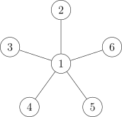
We find that when a node has multiple children with similar \(\mathit{size}\), applying edge decomposition leads to unacceptable time complexity.
If the graph is a binary tree, the drawback of edge decomposition in the star graph can be avoided. Therefore, we consider transforming a multi-way tree into a binary tree.
Clearly, we can construct it similarly to how a segment tree is built, like this:
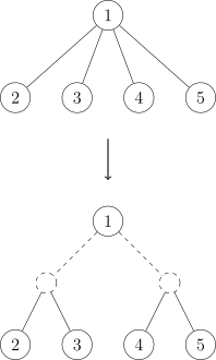
Assign appropriate information to the newly created nodes according to the problem requirements. For example: when counting path lengths, assign weight \(1\) to original edges and weight \(0\) to newly created edges.
Analyzing the complexity, we find that at most \(O(n)\) additional nodes are added, so the total complexity is \(O(n\log n)\).
Almost all problems solvable by centroid decomposition can also be solved by edge decomposition (with constant factor differences, but usually not a bottleneck), so no separate examples are provided here.
Centroid Tree
A centroid tree is a reconstructed tree that changes the original tree's structure to achieve a stable \(\log n\) depth.
It is commonly used to solve dynamic problems unrelated to the original tree structure.
Algorithm Analysis
We reconstruct the original tree by repeatedly finding centroids through centroid decomposition.
Connect each found centroid as a child to the centroid from the previous layer, forming a tree of depth \(\log n\).
Since the tree has \(\log n\) layers, many brute-force approaches that were originally inefficient become feasible with correct complexity on the centroid tree.
Implementation
A small trick: each time, subtract the heavy child size of the node from the previous layer's total size \(\mathit{tot}\) to obtain the total size for the current layer. This way, finding the centroid requires only one DFS.
Reference Code
1 2 3 4 5 6 7 8 9 10 11 12 13 14 15 16 17 18 19 20 21 22 23 24 25 26 27 28 29 30 31 32 33 34 35 36 37 38 39 40 41 42 43 44 45 46 47 48 49 50 51 52 53 54 55 56 57 58 59 60 61 62 63 64 65 66 67 68 69 70 71 72 73 74 75 76 77 78 79 80 | |
本页面最近更新:,更新历史
发现错误?想一起完善? 在 GitHub 上编辑此页!
本页面贡献者:OI-wiki
本页面的全部内容在 CC BY-SA 4.0 和 SATA 协议之条款下提供,附加条款亦可能应用