Binary Search Trees & Balanced Trees
Definition
A Binary Search Tree (BST) is a tree-shaped data structure of a binary tree, defined as follows:
-
An empty tree is a binary search tree.
-
If the left subtree of a binary search tree is not empty, then the additional weights of all nodes on the left subtree are less than the value of its root node.
-
If the right subtree of a binary search tree is not empty, then the additional weights of all nodes on the right subtree are greater than the value of its root node.
-
Both the left and right subtrees of a binary search tree are binary search trees.
The time spent on basic operations on a binary search tree is proportional to the height of the tree. For a binary search tree with \(n\) nodes, the optimal time complexity of these operations is \(O(\log n)\), and the worst-case is \(O(n)\). The expected height of a randomly constructed binary search tree is \(O(\log n)\).
Process
Definition of a Binary Search Tree Node
Implementation
1 2 3 4 5 6 7 8 9 10 11 | |
Traversing a Binary Search Tree
From the recursive definition of a binary search tree, the in-order traversal sequence of the weights of a binary search tree is non-decreasing. The time complexity is \(O(n)\).
The code to traverse a binary search tree is as follows:
Implementation
1 2 3 4 5 6 7 8 | |
Finding Minimum/Maximum Values
From the properties of a binary search tree, the minimum value on a binary search tree is the vertex of the left chain, and the maximum value is the vertex of the right chain. The time complexity is \(O(h)\).
Implementation
1 2 3 4 5 6 7 8 9 10 11 12 13 14 15 16 17 18 19 | |
Searching for an Element
Search for a node with value value in the binary search tree rooted at root.
The classification is as follows:
- If
rootis empty, returnfalse. - If the weight of
rootequalsvalue, returntrue. - If the weight of
rootis greater thanvalue, continue searching in the left subtree ofroot. - If the weight of
rootis less thanvalue, continue searching in the right subtree ofroot.
The time complexity is \(O(h)\).
Implementation
1 2 3 4 5 6 7 8 9 10 11 12 | |
Insertion, deletion, and modification all require searching in the binary search tree first.
Inserting an Element
Insert a node with value value into the binary search tree rooted at root.
The classification is as follows:
-
If
rootis empty, directly return a new node with valuevalue. -
If the weight of
rootequalsvalue, increment the occurrence count of this value in the node's additional field by \(1\). -
If the weight of
rootis greater thanvalue, insert a node with weightvalueinto the left subtree ofroot. -
If the weight of
rootis less thanvalue, insert a node with weightvalueinto the right subtree ofroot.
The time complexity is \(O(h)\).
Implementation
1 2 3 4 5 6 7 8 9 10 11 12 13 14 15 | |
Deleting an Element
Delete a node with value value from the binary search tree rooted at root.
First, search for the node with weight value in the binary search tree. The classification is as follows:
-
If the additional
countof this node is greater than \(1\), only decreasecount. -
If the additional
countof this node is \(1\):-
If
rootis a leaf node, simply delete this node. -
If
rootis a chain node, i.e., a node with only one child, return this child. -
If
roothas two non-empty child nodes, it is generally replaced by the maximum value in its left subtree (the rightmost node of the left subtree) or the minimum value in its right subtree (the leftmost node of the right subtree), and then deleted.
-
Time complexity \(O(h)\).
Implementation
The method uses root = remove(root, 1) to indicate deleting the node with value 1 from the tree rooted at root, and returns the new root node.
1 2 3 4 5 6 7 8 9 10 11 12 13 14 15 16 17 18 19 20 21 22 23 24 25 26 27 28 29 30 31 32 33 34 35 36 37 38 39 40 41 42 43 44 45 46 | |
Finding the Rank of an Element
Rank is defined as the number of numbers before the first identical element after sorting the array elements in ascending order, plus one.
To find the rank of an element, first jump from the root node to this element. If jumping to the right, add the left child node count plus the current node's duplicate count to the answer. Finally, add the size of the left subtree of the destination node plus one to the answer.
Time complexity \(O(h)\).
Implementation
1 2 3 4 5 6 7 | |
Finding the Element with Rank k
In a subtree, the rank of the root node depends on the size of its left subtree.
-
If the size of its left subtree is greater than or equal to \(k\), then the element is in the left subtree;
-
If the size of its left subtree is in the interval \([k-\textit{count},k-1]\) (
countis the occurrence count of the current node's value), then the element is the root node of the subtree; -
If the size of its left subtree is less than \(k-\textit{count}\), then the element is in the right subtree.
Time complexity \(O(h)\).
Implementation
1 2 3 4 5 6 7 8 9 10 11 | |
Introduction to Balanced Trees
One purpose of using search trees is to shorten the time for inserting, deleting, modifying, and searching (insertion, deletion, and modification all include search operations) nodes.
Regarding search efficiency, if the height of a tree is \(h\), in the worst case, searching for a key requires \(h\) comparisons. The search time complexity (also the average search length ASL) does not exceed \(O(h)\). For an ideal binary search tree, all operations can be shortened to \(O(\log n)\) (where n is the total number of nodes).
However, the \(O(\log n)\) time complexity is only ideal. In the worst case, the search tree may degenerate into a linked list. Imagine a binary search tree where each node only has a right child; then its properties are the same as a linked list, and all operations (insert, delete, modify, search) take \(O(n)\) time.
It can be observed that the complexity of operations is related to the height \(h\) of the tree. This leads to balanced trees, which maintain the height (balance) of the tree through certain operations to reduce the complexity of operations.
Definition of Balance
Regarding whether a search tree is "balanced", different balanced trees have different definitions of "balance". For example, for a binary search tree rooted at T, if the heights of the left and right subtrees differ greatly, or the number of nodes in the left subtree is much larger than that in the right subtree, this tree obviously lacks balance.
For binary search trees, a common definition of balance is: for a tree rooted at T, the height difference between the left and right subtrees of every node is at most 1.
-
In a Splay Tree, for any access operation (search, insert, or delete) on a node, the accessed node is moved to the root position of the tree.
-
In an AVL Tree, each node N maintains height information for the tree rooted at N. The definition of balance for an AVL tree: T is an AVL tree if and only if its left and right subtrees are also AVL trees, and \(|height(T->left) - height(T->right)| \leq 1\).
-
In a Size Balanced Tree, each node N maintains the node count
sizeof the tree rooted at N. The definition of balance: thesizeof any node is not less than thesizeof all children (Nephew) of its sibling node (Sibling).
Furthermore, for search trees containing the same set of element values, the balanced state may not be unique. That is, there may be two different search trees containing the same set of element values, and both are balanced.
Balance Adjustment Process
Adjustment operations on a search tree that does not satisfy the balance condition can restore balance to an unbalanced search tree.
Regarding binary balanced trees, balance adjustment operations include Left Rotation (Left Rotate or zag) and Right Rotation (Right Rotate or zig). Since binary balanced trees need to ensure that the in-order traversal sequence remains unchanged during adjustment. Both operations do not change the in-order traversal sequence.
Here, the right rotation is introduced first. Right rotation is also called "right single rotation" or "LL balance rotation". The right rotation operation for node \(A\) means: rotate the left child \(B\) of \(A\) to the upper right, replacing \(A\) as the root node, rotate node \(A\) to the lower right to become the root node of \(B\)'s right subtree, and the original right subtree of \(B\) becomes the left subtree of \(A\).
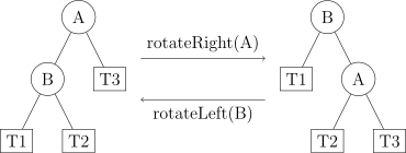
The right rotation operation only changes three sets of node associations, equivalent to a cyclic permutation of three sets of edges, so a node needs to be temporarily stored before performing the rotation update.
For the right rotation operation, the general update order is: temporarily store node \(B\) (the new root node), let \(A\)'s left child point to \(B\)'s right subtree \(T2\), then let \(B\)'s right child pointer point to \(A\), and finally let \(A\)'s parent node point to the temporarily stored \(B\).
Completely similarly, there is a corresponding left rotation operation, also called "left single rotation" or "RR balance rotation". The left rotation operation is the mirror image of the right rotation operation.
The code for left and right rotations is given below.
Implementation
1 2 3 4 5 6 7 8 9 10 11 12 13 14 15 16 17 18 | |
For this example code, when calling, the parent node pre of root needs to be saved. The method returns a pointer to the new root node, and you only need to point pre to the new root node.
Four Cases of Balance Destruction
Although the definitions of different binary balanced trees vary, the differences between binary balanced trees lie only in the information maintained by nodes and the information updated after rotation adjustments. There are only the following four cases where the balance of a binary balanced tree is destroyed. Balance adjustment operations only include left and right rotations. The four cases are introduced first, followed by a comparison of different binary balanced trees.
LL type: The left subtree of T's left child is too long, causing balance destruction.
Adjustment method: Right rotate node T.
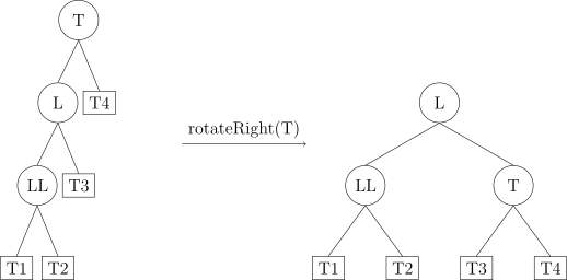
RR type: Similar to LL type, the right subtree of T's right child is too long, causing balance destruction.
Adjustment method: Left rotate node T.
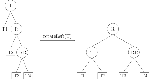
LR type: The right subtree of T's left child is too long, causing balance destruction.
Adjustment method: First left rotate node L, making it an LL type, then right rotate node T.
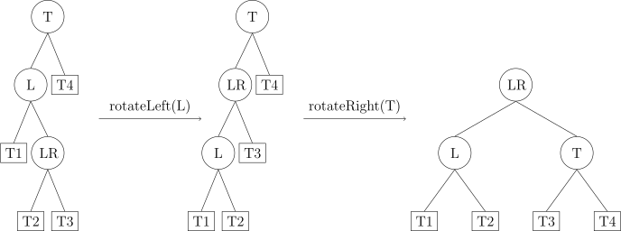
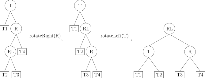
RL type: Similar to LR type, the left subtree of T's right child is too long, causing balance destruction.
Adjustment method: First right rotate node R, making it an RR type, then left rotate node T.
本页面最近更新:,更新历史
发现错误?想一起完善? 在 GitHub 上编辑此页!
本页面贡献者:OI-wiki
本页面的全部内容在 CC BY-SA 4.0 和 SATA 协议之条款下提供,附加条款亦可能应用