Continued Fractions

Introduction

Continued fractions can represent real numbers as the limit of a convergent sequence of rational numbers. The rational numbers in this sequence are easy to compute and provide the best approximations to the real number, so they are often used in algorithm competitions. Additionally, continued fractions are closely related to the Euclidean algorithm and can be applied to a series of number theory problems.

About Algorithm Implementations Related to Continued Fractions

This article will provide a series of algorithm implementations for continued fractions. Some algorithms may not guarantee that the integers involved in intermediate calculations stay within the range of 32-bit or 64-bit integer variables. For such cases, please refer to the corresponding Python implementations or replace the integer variables in the C++ implementations with high-precision integer classes. To focus on key points, some code in this article may call functions implemented earlier without repeating their implementations.

Continued Fractions

Continued fractions (continued fraction) are themselves a form of notation.

Finite Continued Fractions

For a sequence \(\{a_k\}_{i=0}^n\), the continued fraction \([a_0,a_1,\cdots,a_n]\) represents the expansion

\[ x = a_0+\dfrac{1}{a_1+\dfrac{1}{a_2+\dfrac{1}{\cdots+\dfrac{1}{a_n}}}}. \]

A continued fraction is meaningful if and only if the corresponding expansion is meaningful. These \(a_k\) are called the terms or coefficients of the continued fraction.

Notation

More general continued fractions allow numerators in the expansion to not always be \(1\), and the corresponding continued fraction notation also needs modification, which is beyond the scope of this article. Additionally, some literature writes the first comma "\(,\)" as a semicolon "\(;\)", which has no difference in meaning from the notation used here.

Of course, continued fractions can also be extended to infinite sequences.

Infinite Continued Fractions

For an infinite sequence \(\{a_k\}_{i=0}^\infty\), the continued fraction \([a_0,a_1,\cdots]\) represents the limit

\[ x = \lim_{k\rightarrow\infty} x_k = \lim_{k\rightarrow\infty} [a_0,a_1,\cdots,a_k]. \]

A continued fraction is meaningful if and only if the corresponding limit is meaningful. Here, \(x_k=[a_0,a_1,\cdots,a_k]\) is called the \(k\)-th convergent of \(x\), while \(r_k=[a_k,a_{k+1},\cdots]\) is called the \(k\)-th remainder or complete quotient of \(x\). Correspondingly, the term \(a_k\) is sometimes called the \(k\)-th partial quotient.

Simple Continued Fractions

In number theory, we mainly consider continued fractions whose terms are all integers.

Simple Continued Fractions

For a continued fraction \([a_0,a_1,\cdots]\), if \(a_0\) is an integer and \(a_1,a_2,\cdots\) are all positive integers, it is called a simple continued fraction, also simply referred to as a continued fraction. If the sequence \(\{a_i\}\) is finite, it is called a finite (simple) continued fraction; otherwise, it is called an infinite (simple) continued fraction. Moreover, \(a_0\) is called its integer part.

Unless otherwise specified, the continued fractions mentioned in this article refer to simple continued fractions. It can be proven that infinite simple continued fractions are always convergent, and the remainders of simple continued fractions are always positive.

Continued fractions have the following basic properties:

Properties

Let the real number \(x=[a_0,a_1,a_2,\cdots]\). Then, the following properties hold:

1. For any \(k\in\mathbf Z\), \(x+k=[a_0+k,a_1,a_2,\cdots]\);
2. For a real number \(x>1\), \(a_0>0\), and its reciprocal \(x^{-1}=[0,a_0,a_1,a_2,\cdots]\).

Finite continued fractions correspond to rational numbers. Each rational number has exactly two ways to be represented as a continued fraction, with lengths necessarily one odd and one even. The only difference between these two representations is whether the last term is \(1\), i.e.,

\[ x = [a_0,a_1,\cdots,a_n] = [a_0,a_1,\cdots,a_n-1,1]. \]

These two continued fractions are called the continued fraction representations of the rational number \(x\).[^one-representation] The one with the last term not equal to \(1\) is called the standard representation, and the one with the last term equal to \(1\) is called the non-standard representation.

Example

The continued fraction representation of the rational number \(x=\dfrac{5}{3}\) is

\[ \begin{aligned} x = [1,1,1,1] &= 1+\dfrac{1}{1+\dfrac{1}{1+\dfrac{1}{1}}},\\ x = [1,1,2] &= 1+\dfrac{1}{1+\dfrac{1}{2}}. \end{aligned} \]

Infinite continued fractions correspond to irrational numbers. Moreover, each irrational number has a unique way to be represented as a continued fraction, called the continued fraction representation of the irrational number.

Computing the Continued Fraction Representation

To find the continued fraction representation of a real number \(x\), note that if its remainder \(r_k\) is not an integer, it must satisfy

\[ r_k = [a_k,a_{k+1},\cdots] = [a_k,r_{k+1}] = a_k + \dfrac{1}{r_{k+1}}. \]

Moreover, \(r_{k+1}>1\). Therefore, starting from \(r_0=x\), we can recursively compute

\[ a_k = \lfloor r_k\rfloor,\ r_{k+1} = \dfrac{1}{r_k-a_k}. \]

The sequence \(\{a_k\}\) produced by this process is always uniquely determined, unless some remainder \(r_k\) becomes an integer. If \(r_k\) becomes an integer, the process should terminate, and we can choose to output the corresponding standard or non-standard representation.

In algorithm competitions, we often deal with rational numbers \(x=\dfrac{p}{q}\). In this case, each remainder \(r_k\) is a rational number \(\dfrac{p_k}{q_k}\), and for \(k>0\), since \(r_k>1\), we always have \(p_k>q_k\). Specifically computing the above recurrence relation, we find

\[ a_k = \left\lfloor\frac{p_k}{q_k}\right\rfloor,\ r_{k+1} = \dfrac{1}{r_k-a_k} = \dfrac{q_k}{p_k-a_kq_k} = \dfrac{q_k}{p_k\bmod q_k}. \]

At this point, the computation process is essentially performing the Euclidean algorithm on \(p\) and \(q\). This also shows that for a rational number \(r=\dfrac{p}{q}\), the length of its continued fraction representation is \(O(\log\min\{p, q\})\). The complexity of computing the continued fraction representation of \(\dfrac{p}{q}\) is also \(O(\log\min\{p, q\})\).

Reference Implementation

Given the numerator \(p\) and denominator \(q\) of a fraction, output the coefficient sequence \([a_0,a_1,\cdots,a_n]\) of its continued fraction.

C++Python

// Find the continued fraction representation of P/Q.
auto fraction(int p, int q) {
  std::vector<int> a;
  while (q) {
    a.push_back(p / q);
    std::tie(p, q) = std::make_pair(q, p % q);
  }
  return a;
}

# Find the continued fraction representation of P/Q.
def fraction(p, q):
    a = []
    while q:
        a.append(p // q)
        p, q = q, p % q
    return a

Convergents

The concept of convergents was introduced in the definition of continued fractions. The convergents of a real number are the convergents of its continued fraction representation: in the continued fraction representation of a real number \(x\), keeping only the first \(k\) terms yields the continued fraction \(x_k\), called the \(k\)-th convergent of the real number \(x\). The convergents \(x_k\) of a real number \(x\) are all rational numbers, and the sequence \(\{x_k\}\) converges to the real number \(x\).

Example: Convergents of the Golden Ratio

The first few convergents of the continued fraction \(x=[1,1,1,1,\cdots]\) are

\[ \begin{aligned} x_0 &= [1]=1,\\ x_1 &= [1,1]=2,\\ x_2 &= [1,1,1]=\dfrac{3}{2},\\ x_3 &= [1,1,1,1]=\dfrac{5}{3},\\ x_4 &= [1,1,1,1,1]=\dfrac{8}{5}. \end{aligned} \]

It can be proven by induction that

\[ x_k = \frac{F_{k+2}}{F_{k+1}}, \]

where \(\{F_k\}\) is the Fibonacci sequence. According to its closed-form formula,

\[ x_k = \frac{\phi^{k+2}-(-\phi)^{-(k+2)}}{\phi^{k+1}-(-\phi)^{-(k+1)}}, \]

where \(\phi=\dfrac{1+\sqrt{5}}{2}\) is the golden ratio. As \(k\) tends to infinity,

\[ x=\lim_{k\rightarrow\infty}x_k=\phi. \]

Thus, the continued fraction \(x=[1,1,1,1,\cdots]\) represents the golden ratio \(\phi\).

These convergents approach the corresponding real number, so they can be used to approximate that real number. For this purpose, it is necessary to understand the properties of convergents.

Recurrence Relations

First, we need to address the computation of these convergents. Although convergents are always obtained by adding one term to the continued fraction, we do not need to recalculate their values each time. In fact, convergents have the following recurrence relation:

Recurrence Formula

For a continued fraction \(x=[a_0,a_1,a_2,\cdots]\), let its \(k\)-th convergent \(x_k\) be written as the fraction \(\dfrac{p_k}{q_k}\). Then,

\[ \begin{aligned} p_k &= a_kp_{k-1}+p_{k-2},\\ q_k &= a_kq_{k-1}+q_{k-2}. \end{aligned} \]

The starting points of the recurrence are the (formal) fractions

\[ x_{-1}=\frac{p_{-1}}{q_{-1}}=\frac{1}{0},\ x_{-2}=\frac{p_{-2}}{q_{-2}}=\frac{0}{1}. \]

Proof

The numerator and denominator of the convergent \(x_k\) can be viewed as multivariate polynomials in \(a_0, a_1, \cdots, a_k\):

\[ r_k = \frac{P_k(a_0, a_1, \cdots, a_k)}{Q_k(a_0,a_1, \cdots, a_k)}. \]

According to the definition of convergents,

\[ r_k = a_0 + \frac{1}{[a_1,a_2,\cdots, a_k]}= a_0 + \frac{Q_{k-1}(a_1, \cdots, a_k)}{P_{k-1}(a_1, \cdots, a_k)} = \frac{a_0 P_{k-1}(a_1, \dots, a_k) + Q_{k-1}(a_1, \cdots, a_k)}{P_{k-1}(a_1, \cdots, a_k)}. \]

Comparing with the above expression, we can set \(Q_k(a_0, \cdots, a_k) = P_{k-1}(a_1, \cdots, a_k)\), so the convergent can be written as

\[ r_k = \frac{P_k(a_0, a_1, \cdots, a_k)}{P_{k-1}(a_1, \cdots, a_k)} \]

and the polynomial \(P_k\) has the recurrence relation

\[ P_k(a_0, \cdots, a_k) = a_0 P_{k-1}(a_1, \cdots, a_k) + P_{k-2}(a_2, \cdots, a_k). \]

Since

\[ r_0 = a_0,\ r_1 = a_0+\dfrac{1}{a_1} = \frac{a_0a_1+1}{a_1}, \]

the starting points of the recurrence are

\[ P_0(a_0) = a_0,\ P_1(a_0,a_1) = a_0a_1 + 1. \]

If we set

\[ P_{-1} = 1,\ P_{-2} = 0, \]

we can verify that the above recurrence relation also holds for \(k=0,1\). This is equivalent to defining the formal fractions \(r_{-1}=\dfrac{1}{0}\) and \(r_{-2}=\dfrac{0}{1}\).

The polynomial sequence \(P_k\) satisfying the above recurrence relation is called continuant[^continuant]. It can be written in determinant form:

\[ P_k(a_0,\cdots,a_k)=\det \begin{pmatrix} a_0 & 1 & 0 & \cdots & 0 \\ -1 & a_1 & 1 & \ddots & \vdots \\ 0 & -1 & a_2 & \ddots & 0 \\ \vdots & \ddots & \ddots & \ddots & 1 \\ 0 & \cdots & 0 & -1 & a_k \end{pmatrix}. \]

This is the determinant of a tridiagonal matrix. Expanding from the top-left corner, we can verify that it has the above recurrence relation and initial conditions. Conversely, expanding from the bottom-right corner yields the recurrence relation

\[ P_k(a_0, \cdots, a_k) = a_k P_{k-1}(a_0, \cdots, a_{k-1}) + P_{k-2}(a_0, \cdots, a_{k-2}), \]

which is exactly what we wanted to prove.

Notation

When writing the convergent \(x_k\) as \(\dfrac{p_k}{q_k}\) in this article, it is always assumed that the numerator \(p_k\) and denominator \(q_k\) are given by the recurrence relation above. It will be shown later that this always yields the reduced form of the convergent.

This recurrence implies that

\[ x_k=\dfrac{a_kp_{k-1}+p_{k-2}}{a_kq_{k-1}+q_{k-2}} \]

lies between \(x_{k-1}\) and \(x_{k-2}\).

As a corollary of the recurrence relation for convergents, we have the following reversal theorem and reciprocal theorem:

Reversal Theorem

Let the \(k\)-th convergent of the real number \(x=[a_0,a_1,a_2,\cdots]\) be \(\dfrac{p_k}{q_k}\). Then, the ratios of the numerators and denominators of adjacent convergents are

\[ \begin{aligned} \frac{p_k}{p_{k-1}}&=[a_k,a_{k-1},\cdots,a_1,a_0],\\ \frac{q_k}{q_{k-1}}&=[a_k,a_{k-1},\cdots,a_1]. \end{aligned} \]

If \(a_0=0\), the first continued fraction should be understood as truncated at the second-to-last term, i.e., \([a_k,a_{k-1},\cdots,a_2]\).

Proof

In the recurrence relations for \(p_k\) and \(q_k\), dividing both sides by \(p_{k-1}\) and \(q_{k-1}\) respectively, we get

\[ \begin{aligned} \frac{p_k}{p_{k-1}} &= a_k + \frac{p_{k-2}}{p_{k-1}},\\ \frac{q_k}{q_{k-1}} &= a_k + \frac{q_{k-2}}{q_{k-1}}. \end{aligned} \]

Iterating these two equations yields two continued fractions. Substituting the initial values \(\dfrac{p_0}{p_{-1}}=a_0\) and \(\dfrac{q_1}{q_0}=a_1\) completes the proof. For the case \(a_0=0\), interpreting the obtained continued fraction as a formal expression, its remainder

\[ [a_2,a_1,0]=a_2+\dfrac{1}{a_1+\dfrac{1}{0}}=a_2+\dfrac{0}{0a_1+1}=a_2. \]

Thus, the last two terms can be directly omitted. If a rigorous proof is needed, note that this expression can be viewed as the limit as \(a_0\rightarrow 0\).

Reciprocal Theorem

The reciprocal of a convergent of a real number \(x>0\) is a convergent of \(x^{-1}\).

Proof

Assume \(x>1\) and has continued fraction representation \([a_0,a_1,a_2,\cdots]\). Then, the continued fraction representation of \(x^{-1}\) is \([0,a_0,a_1,a_2,\cdots]\). Their convergents can be obtained from the recurrence relations. For \(x\), the initial conditions are \(x_{-2}=\dfrac{0}{1}\) and \(x_{-1}=\dfrac{1}{0}\); for \(y=x^{-1}\), the initial conditions are \(y_{-1}=\dfrac{1}{0}\) and \(y_{0}=\dfrac{0}{1}\). Therefore, \(x_{-2}=(y_{-1})^{-1}\) and \(x_{-1}=(y_0)^{-1}\). By the recurrence relation, we get \(x_k=y_{k+1}^{-1}\). This shows that the reciprocal of a convergent of \(x\) is a convergent of \(y=x^{-1}\). A similar discussion applies to the case \(0<x\le 1\).

Using the recurrence relation obtained in this section, we can derive the following algorithm for computing convergents:

Reference Implementation

Given the coefficients \(a_0,a_1,\cdots,a_n\) of a continued fraction, find the numerator and denominator sequences \((p_0,q_0),(p_1,q_1),\cdots,(p_n,q_n)\) of its convergents.

C++Python

// Find the convergents of a continued fraction A.
// Numerators and denominators stored separately in P and Q.
auto convergents(std::vector<int> a) {
  std::vector<int> p = {0, 1};
  std::vector<int> q = {1, 0};
  for (auto it : a) {
    p.push_back(p.back() * it + p.end()[-2]);
    q.push_back(q.back() * it + q.end()[-2]);
  }
  return std::make_pair(p, q);
}

# Find the convergents of a continued fraction A.
# Numerators and denominators stored separately in P and Q.
def convergents(a):
    p = [0, 1]
    q = [1, 0]
    for it in a:
        p.append(p[-1] * it + p[-2])
        q.append(q[-1] * it + q[-2])
    return p, q

Error Estimation

Using the recurrence formula for convergents, we can estimate the error when approximating a real number with convergents.

First, we can compute the difference between adjacent convergents:

Difference of Convergents

Let \(x_k=\dfrac{p_k}{q_k}\) be the \(k\)-th convergent of the real number \(x\). Then,

\[ p_{k+1}q_k − p_kq_{k+1} = (−1)^k. \]

Therefore, the difference between two adjacent convergents is

\[ x_{k+1} - x_k = \dfrac{(-1)^k}{q_{k+1}q_k}. \]

Proof

According to the recurrence relation,

\[ \begin{aligned} \det\begin{pmatrix} p_{k+1} & p_k \\ q_{k+1} & q_k \end{pmatrix} &= \det\begin{pmatrix} a_{k+1}p_{k}+p_{k-1} & p_k \\ a_{k+1}q_{k}+q_{k-1} & q_k \end{pmatrix} = \det\begin{pmatrix} p_{k-1} & p_k\\ q_{k-1} & q_k \end{pmatrix} \\ &= - \det\begin{pmatrix} p_k & p_{k-1}\\ q_k & q_{k-1} \end{pmatrix} = (-1)^{k+2} \det\begin{pmatrix} 1 & 0\\ 0 & 1 \end{pmatrix} =(-1)^k. \end{aligned} \]

This gives \(p_{k+1}q_k − p_kq_{k+1} = (−1)^k\). Dividing both sides by \(q_{k+1}q_k\) yields the conclusion about \(x_{k+1}-x_k\).

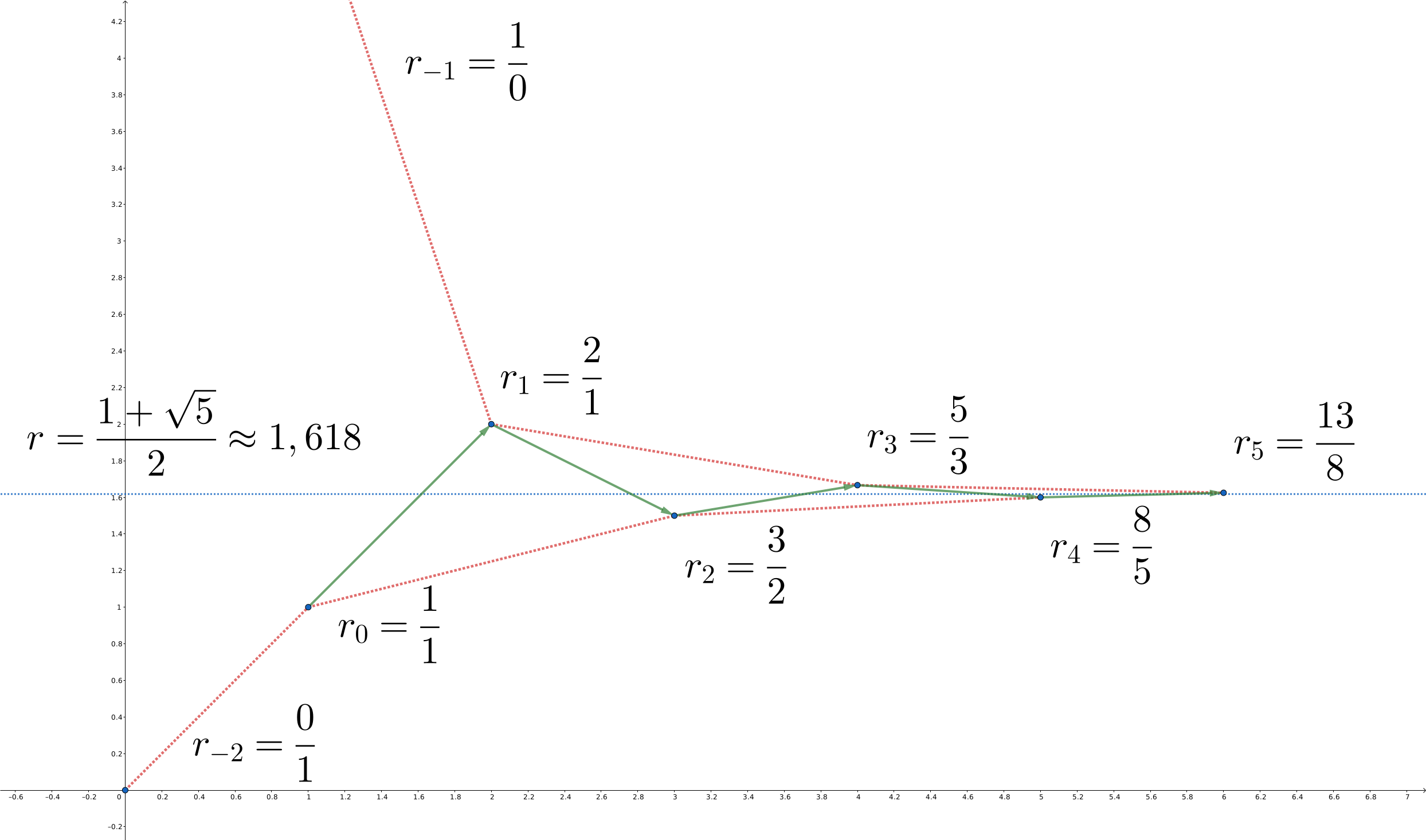
Thus, odd-indexed convergents are always greater than their adjacent terms, and even-indexed convergents are always less than their adjacent terms: convergents alternate.

If we only consider even-indexed (or odd-indexed) convergents, the sequence is also monotonically increasing (or decreasing). This is because

\[ x_{k+2}-x_k = \dfrac{(-1)^{k+1}}{q_{k+2}q_{k+1}}+\dfrac{(-1)^{k}}{q_{k+1}q_{k}} = \dfrac{(-1)^k(q_{k+2}-q_k)}{q_{k+2}q_{k+1}q_k} = \dfrac{(-1)^ka_{k+2}}{q_{k+2}q_k} \]

is positive when \(k\) is even (odd). At the same time, since the recurrence \(q_{k}=a_kq_{k-1}+q_{k-2}\) holds, the denominator \(q_k\) grows at least as fast as the Fibonacci sequence. Therefore, the difference between adjacent terms must tend to zero. This shows that the even-indexed and odd-indexed convergents approach the same limit from below and above, respectively. This proves that infinite simple continued fractions always converge. The dynamics of convergents approaching the corresponding real number can be seen in the figure below:

Upper (Lower) Convergent

For a real number \(x\) and its convergent \(x_k\), if \(x_k>x\) (\(x_k<x\)), then \(x_k\) is called an upper (lower) convergent of \(x\).

As already shown, upper convergents are the odd-indexed convergents, and lower convergents are the even-indexed convergents.

Using the difference formula, we can write the real number \(x\) as an alternating series:

\[ x = a_0+\sum_{k=0}^{\infty}\dfrac{(-1)^k}{q_{k+1}q_k}. \]

The convergents and remainders in the definition of continued fractions are the partial sums and remainder of this series.

Using the difference formula, we can also directly estimate the error when approximating a real number with convergents:

Error

Let \(x_k=\dfrac{p_k}{q_k}\neq x\) be the \(k\)-th convergent of the real number \(x\). Then,

\[ x_k - x = \dfrac{(-1)^k}{q_k\left(r_{k+1}q_k+q_{k-1}\right)}, \]

where \(r_{k+1}\) is the \((k+1)\)-th remainder of the real number \(x\). Furthermore,

\[ \dfrac{1}{2q_{k+1}^2} \le \dfrac{1}{q_k(q_k+q_{k+1})} \le \left|x-\frac{p_k}{q_k}\right| \le \dfrac{1}{q_kq_{k+1}} \le \dfrac{1}{q_k^2}. \]

Proof

Since \(x=[a_0,a_1,\cdots,a_k,r_{k+1}]\), and the difference formula for convergents also holds for formal continued fractions, we have

\[ x-x_k = \dfrac{(-1)^k}{q_k\left(r_{k+1}q_k+q_{k-1}\right)}, \]

where \(r_{k+1}q_k+q_{k-1}\) is the denominator of the \((k+1)\)-th convergent of this formal continued fraction obtained via the recurrence formula.

To complete the subsequent inequality estimates, note that when \(x_k\neq x\), we always have

\[ 1\le a_{k+1}\le r_{k+1} \le a_{k+1}+1, \]

so

\[ q_{k+1}=a_{k+1}q_k+q_{k-1}\le r_{k+1}q_k+q_{k-1} \le q_k+(a_{k+1}q_k+q_{k-1}) = q_k+q_{k+1}. \]

Therefore, we have the inequality

\[ \dfrac{1}{q_k(q_k+q_{k+1})} \le \left|x-\frac{p_k}{q_k}\right| = \dfrac{1}{q_k\left(r_{k+1}q_k+q_{k-1}\right)} \le \dfrac{1}{q_kq_{k+1}}. \]

To obtain the outer bounds, note that \(q_k\le q_{k+1}\).

A simple corollary of the difference formula in this section is that the convergents \(\dfrac{p_k}{q_k}\) are all in reduced form.

Corollary

For any real number \(x\), with the numerator and denominator of the convergent \(x_k=\dfrac{p_k}{q_k}\) given by the recurrence formula, \(\dfrac{p_k}{q_k}\) is a reduced fraction, i.e., \(\gcd(p_k,q_k)=1\).

Proof

Apply Bézout's theorem to the difference formula.

In fact, solutions to binary linear Diophantine equations can be found using continued fractions.

Solving Binary Linear Diophantine Equations

Given \(A, B, C \in \mathbf Z\). Find \(x, y \in \mathbf Z\) such that \(Ax + By = C\).

Solution

Although this problem is usually solved using the extended Euclidean algorithm, it can also be solved via continued fractions.

Let \(\dfrac{A}{B}=[a_0, a_1, \cdots, a_k]\). It was shown above that \(p_k q_{k-1} - p_{k-1} q_k = (-1)^{k-1}\). Replacing \(p_k\) and \(q_k\) with \(A\) and \(B\), we get

\[ Aq_{k-1} - Bp_{k-1} = (-1)^{k-1} g, \]

where \(g = \gcd(A, B)\). If \(g\) divides \(C\), then one solution is \(x = (-1)^{k-1}\dfrac{C}{g} q_{k-1}\) and \(y = (-1)^{k}\dfrac{C}{g} p_{k-1}\); otherwise, there is no solution.

C++Python

// Return (x,y) such that Ax+By=C.
// Assume that such (x,y) exists.
auto dio(int A, int B, int C) {
  std::vector<int> p, q;
  std::tie(p, q) = convergents(fraction(A, B));
  C /= A / p.back();
  int t = p.size() % 2 ? -1 : 1;
  return std::make_pair(t * C * q.end()[-2], -t * C * p.end()[-2]);
}

# Return (x, y) such that Ax+By=C.
# Assume that such (x, y) exists.
def dio(A, B, C):
    p, q = convergents(fraction(A, B))
    C //= A // p[-1]  # divide by gcd(A, B)
    t = (-1) if len(p) % 2 else 1
    return t * C * q[-2], -t * C * p[-2]

Diophantine Approximation

An important application of continued fraction theory is Diophantine approximation theory. Diophantine approximation refers to approximating real numbers with rational numbers. Of course, due to the density of rational numbers, without restrictions, we can obtain approximations with arbitrarily small error. Therefore, restrictions must be placed on the rational numbers used, such as only choosing rational numbers with denominators less than a certain value. This section discusses the relationship between best approximations under such restrictions and continued fractions.

Approximating Real Numbers with Convergents

First, using the error estimate for convergents, we immediately obtain the following result:

Theorem (Dirichlet)

For an irrational number \(x\), there exist infinitely many reduced fractions \(\dfrac{p}{q}\) such that

\[ \left|x-\dfrac{p}{q}\right| < \dfrac{1}{q^2} \]

holds.

Proof

According to the error estimate for convergents, for the \(k\)-th convergent \(x_k=\dfrac{p_k}{q_k}\) of the irrational number \(x\), we have

\[ \left|x-\dfrac{p_k}{q_k}\right|\le\frac{1}{q_k^2}. \]

Examining the proof of the error formula shows that equality does not hold for any irrational number \(x\). Therefore, the numerators and denominators of all its convergents satisfy the requirement.

This theorem can also be seen as a corollary of Dirichlet's approximation theorem. This is almost the best possible result. The exponent \(2\) in the denominator on the right side of the inequality cannot be improved, but the constant can be made better. Hurwitz's theorem states that the right side can be reduced to \(\dfrac{1}{\sqrt{5}q^2}\), and this is the best bound.

Hurwitz Theorem

For an irrational number \(x\), there exist infinitely many reduced fractions \(\dfrac{p}{q}\) such that

\[ \left|x-\dfrac{p}{q}\right| < \dfrac{1}{\sqrt{5}q^2} \]

holds, and the \(\sqrt{5}\) on the right side cannot be replaced by a larger real number.

Proof (Borel)

Borel actually proved that among three consecutive convergents of an irrational number \(x\), at least one must satisfy the above condition. Since there are infinitely many convergents, all of which are reduced fractions, the first part of Hurwitz's theorem necessarily holds.

By contradiction. Suppose there exists an irrational number \(x\) and its convergents \(x_{k-1},x_k,x_{k+1}\) such that

\[ \left|x-\dfrac{p_{k-1}}{q_{k-1}}\right|\ge\dfrac{1}{\sqrt{5}q_{k-1}^2},\ \left|x-\dfrac{p_{k}}{q_{k}}\right|\ge\dfrac{1}{\sqrt{5}q_{k}^2},\ \left|x-\dfrac{p_{k+1}}{q_{k+1}}\right|\ge\dfrac{1}{\sqrt{5}q_{k+1}^2} \]

hold. Since adjacent convergents must lie on opposite sides of \(x\), by the difference formula,

\[ \dfrac{1}{q_{k-1}q_{k}}=\left|\dfrac{p_{k-1}}{q_{k-1}}-\dfrac{p_{k}}{q_{k}}\right|=\left|x-\dfrac{p_{k-1}}{q_{k-1}}\right|+\left|x-\dfrac{p_{k}}{q_{k}}\right|\ge\dfrac{1}{\sqrt{5}q_{k-1}^2}+\dfrac{1}{\sqrt{5}q_{k}^2}. \]

This can be written as an inequality about the ratio \(\dfrac{q_{k}}{q_{k-1}}\):

\[ \dfrac{q_k}{q_{k-1}}+\dfrac{q_{k-1}}{q_k}\le\sqrt 5. \]

Since the left side is rational and the right side is irrational, equality cannot hold. Also, since \(q_k\ge q_{k-1}\), we can solve

\[ 1\le \dfrac{q_{k}}{q_{k-1}} < \dfrac{\sqrt{5}+1}{2}. \]

Similarly, we can prove

\[ 1\le \dfrac{q_{k+1}}{q_{k}} < \dfrac{\sqrt{5}+1}{2}. \]

But according to the recurrence relation and combining the two inequalities,

\[ a_{k+1} = \frac{q_{k+1}}{q_k}-\frac{q_{k-1}}{q_k} < \dfrac{\sqrt{5}+1}{2}-\dfrac{\sqrt{5}-1}{2} = 1 \]

which contradicts the definition of a simple continued fraction. Thus, Borel's conclusion holds.

To show that the bound obtained is the best, we need to find an \(x\) such that for any \(C>\sqrt{5}\), there are only finitely many reduced fractions \(\dfrac{p}{q}\) satisfying

\[ \left|x-\dfrac{p}{q}\right| < \dfrac{1}{Cq^2} \]

We now prove that \(\phi=\dfrac{\sqrt{5}+1}{2}\) is such an \(x\).[^sqrt5]

Let \(\phi'=\dfrac{-\sqrt{5}+1}{2}\) be the conjugate of \(\phi\). Both are roots of the equation \(x^2-x-1=0\). Thus, for any real number \(x\),

\[ x^2-x-1 = (x-\phi)(x-\phi'). \]

Substituting a reduced fraction \(\dfrac{p}{q}\), we get

\[ \dfrac{1}{q^2}\le\frac{|p^2-pq-q^2|}{q^2}=\left|\dfrac{p}{q}-\phi\right|\left|\dfrac{p}{q}-\phi'\right|\le\left|\dfrac{p}{q}-\phi\right|\left(\left|\dfrac{p}{q}-\phi\right|+|\phi-\phi'|\right)<\dfrac{1}{Cq^2}\left(\dfrac{1}{Cq^2}+\sqrt{5}\right). \]

For \(C>\sqrt{5}\), we can directly solve \(q<\sqrt{C(C-\sqrt{5})}\), so there cannot be infinitely many solutions satisfying the inequality.

The proofs of these theorems show that convergents provide very good Diophantine approximations. However, they may not be the best approximations. To discuss best approximations, we need to specify the measure of approximation quality. There are often two choices.

Cases Where Best Approximation Results May Not Hold

The next two sections will present some results about best approximations. These results may not hold for some trivial cases. For example, both definitions of best approximations require strict inequalities, but for a half-integer \(x=n+\dfrac12\) with \(n\in\mathbf Z\), its continued fraction form can be \([n,1,1]\). In this case, its first two convergents \(x_0=n\) and \(x_1=n+1\) both have denominator \(1\) and are equidistant from \(x\). This shows that neither is a best approximation. For the statements in this section, readers should assume such cases are excluded. If readers are not concerned with the last few convergents or only care about approximations of irrational numbers, they can ignore these additional complexities.

Best Approximations of the First Kind: Intermediate Fractions

Best approximations of the first kind use

\[ \left|x-\dfrac{p}{q}\right| \]

to measure the quality of approximation.

Best Approximation of the First Kind

For a real number \(x\) and a rational number \(\dfrac{p}{q}\), if for any \(\dfrac{p'}{q'}\neq \dfrac{p}{q}\) with \(0<q'\le q\) we have

\[ \left|x-\dfrac{p}{q}\right|<\left|x-\dfrac{p'}{q'}\right|, \]

then the rational number \(\dfrac{p}{q}\) is called a best approximation of the first kind to the real number \(x\).

Best approximations of the first kind are not necessarily convergents but a broader class of fractions.

Intermediate Fractions

Let the real number \(x\) have convergents \(x_{k+1}=[a_0,a_1,\cdots,a_k,a_{k+1}]\), and let integer

---

本页面最近更新：，更新历史
发现错误？想一起完善？ 在 GitHub 上编辑此页！
本页面贡献者：OI-wiki
本页面的全部内容在 CC BY-SA 4.0 和 SATA 协议之条款下提供，附加条款亦可能应用