Maximum General Graph Matching

Blossom Algorithm

The Blossom Algorithm (also known as the Blossom Tree Algorithm) can solve the maximum cardinality matching problem in general graphs. This algorithm was proposed by Jack Edmonds in 1961. With some modifications, it can also solve the maximum weight matching problem in general graphs. This algorithm was the first to prove that maximum matching has polynomial complexity.

The difference between general graph matching and bipartite matching is that the graph may contain odd cycles.

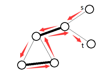
Taking this graph as an example, if we directly invert (swap matched and unmatched edges), the resulting \(M\) would be invalid, as some vertices would appear in two matched edges. The problem lies in the odd cycle.

Now consider the augmenting path algorithm for general graphs. From the perspective of bipartite graphs, each time we enumerate an unmatched vertex, set it as the root, and mark it as "o". Then alternately mark "o" and "i". It is not difficult to see that the edges from "i" to "o" are matched edges.

Assume the current vertex is \(v\), and its adjacent vertex is \(u\). There are two cases:

1. \(u\) has not been visited. If \(u\) is unmatched, then an augmenting path is found; otherwise, search for an augmenting path from \(u\)'s partner.
2. \(u\) has been visited. If the mark is "o", it indicates the need for blossom contraction; otherwise, it indicates an even cycle, which can be skipped.

For even cycles, treat them as bipartite graphs, so they can be ignored. After blossom contraction, continue searching for augmenting paths in the new graph.

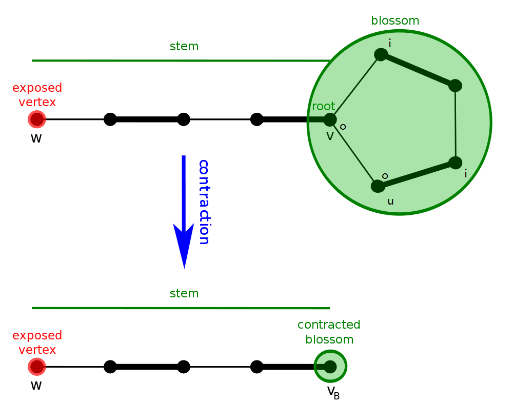
Let the original graph be \(G\), and the graph after blossom contraction be \(G'\). We only need to prove:

1. If \(G\) has an augmenting path, then \(G'\) also has one.
2. If \(G'\) has an augmenting path, then \(G\) also has one.

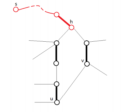
Let the non-tree edge (the edge forming the cycle) be \((u,v)\), and define the blossom root \(h=LCA(u,v)\). The odd cycle alternates, and only the two edges adjacent to \(h\) are of the same type, both unmatched edges. Thus, the tree edge entering \(h\) must be a matched edge, and all vertices on the cycle except \(h\) have unmatched edges connecting to the outside of the cycle.

Observing the graph, there are two ways to exit the cycle from an external edge: clockwise or counterclockwise.

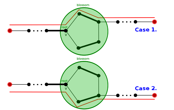
Therefore, whether blossom contraction is performed or not does not affect correctness.

In practice, after finding a blossom, we do not need to actually contract it. Instead, we can use an array to record which blossom root each vertex belongs to.

Complexity Analysis

Each time an augmenting path is searched, all edges are traversed. When encountering a blossom, the vertices on the blossom are maintained, resulting in \(O(|E|^2)\).

Enumerating all unmatched vertices to find augmenting paths yields a total complexity of \(O(|V||E|^2)\).

Reference Code

Reference Code

// graph
template <typename T>
class graph {
 public:
  struct edge {
    int from;
    int to;
    T cost;
  };

  vector<edge> edges;
  vector<vector<int>> g;
  int n;

  graph(int _n) : n(_n) { g.resize(n); }

  virtual int add(int from, int to, T cost) = 0;
};

// undirectedgraph
template <typename T>
class undirectedgraph : public graph<T> {
 public:
  using graph<T>::edges;
  using graph<T>::g;
  using graph<T>::n;

  undirectedgraph(int _n) : graph<T>(_n) {}

  int add(int from, int to, T cost = 1) {
    assert(0 <= from && from < n && 0 <= to && to < n);
    int id = (int)edges.size();
    g[from].push_back(id);
    g[to].push_back(id);
    edges.push_back({from, to, cost});
    return id;
  }
};

// blossom / find_max_unweighted_matching
template <typename T>
vector<int> find_max_unweighted_matching(const undirectedgraph<T> &g) {
  std::mt19937 rng(std::random_device{}());
  vector<int> match(g.n, -1);   // matching
  vector<int> aux(g.n, -1);     // timestamp
  vector<int> label(g.n);       // "o" or "i"
  vector<int> orig(g.n);        // blossom root
  vector<int> parent(g.n, -1);  // parent vertex
  queue<int> q;
  int aux_time = -1;

  auto lca = [&](int v, int u) {
    aux_time++;
    while (true) {
      if (v != -1) {
        if (aux[v] == aux_time) {  // found visited vertex, i.e., LCA
          return v;
        }
        aux[v] = aux_time;
        if (match[v] == -1) {
          v = -1;
        } else {
          v = orig[parent[match[v]]];  // continue searching from the parent of the matched vertex
        }
      }
      swap(v, u);
    }
  };  // lca

  auto blossom = [&](int v, int u, int a) {
    while (orig[v] != a) {
      parent[v] = u;
      u = match[v];
      if (label[u] == 1) {  // set initial point as "o" to find augmenting path
        label[u] = 0;
        q.push(u);
      }
      orig[v] = orig[u] = a;  // contract blossom
      v = parent[u];
    }
  };  // blossom

  auto augment = [&](int v) {
    while (v != -1) {
      int pv = parent[v];
      int next_v = match[pv];
      match[v] = pv;
      match[pv] = v;
      v = next_v;
    }
  };  // augment

  auto bfs = [&](int root) {
    fill(label.begin(), label.end(), -1);
    iota(orig.begin(), orig.end(), 0);
    while (!q.empty()) {
      q.pop();
    }
    q.push(root);
    // set initial point as "o", here "0" represents "o", "1" represents "i"
    label[root] = 0;
    while (!q.empty()) {
      int v = q.front();
      q.pop();
      for (int id : g.g[v]) {
        auto &e = g.edges[id];
        int u = e.from ^ e.to ^ v;
        if (label[u] == -1) {  // found unvisited vertex
          label[u] = 1;        // mark as "i"
          parent[u] = v;
          if (match[u] == -1) {  // found unmatched vertex
            augment(u);          // find augmenting path
            return true;
          }
          // found matched vertex, push its partner into queue to extend alternating tree
          label[match[u]] = 0;
          q.push(match[u]);
          continue;
        } else if (label[u] == 0 && orig[v] != orig[u]) {
          // found visited vertex with same mark "o", indicating a blossom
          int a = lca(orig[v], orig[u]);
          // find LCA and contract blossom
          blossom(u, v, a);
          blossom(v, u, a);
        }
      }
    }
    return false;
  };  // bfs

  auto greedy = [&]() {
    vector<int> order(g.n);
    // randomly shuffle order
    iota(order.begin(), order.end(), 0);
    shuffle(order.begin(), order.end(), rng);

    // match vertices that can be matched
    for (int i : order) {
      if (match[i] == -1) {
        for (auto id : g.g[i]) {
          auto &e = g.edges[id];
          int to = e.from ^ e.to ^ i;
          if (match[to] == -1) {
            match[i] = to;
            match[to] = i;
            break;
          }
        }
      }
    }
  };  // greedy

  // start with random matching
  greedy();
  // find augmenting paths for unmatched vertices
  for (int i = 0; i < g.n; i++) {
    if (match[i] == -1) {
      bfs(i);
    }
  }
  return match;
}

UOJ #79. General Graph Maximum Matching

#include <algorithm>
#include <cassert>
#include <iostream>
#include <numeric>
#include <queue>
#include <random>
#include <vector>
using namespace std;

// graph
template <typename T>
class graph {
 public:
  struct edge {
    int from;
    int to;
    T cost;
  };

  vector<edge> edges;
  vector<vector<int>> g;
  int n;

  graph(int _n) : n(_n) { g.resize(n); }

  virtual int add(int from, int to, T cost) = 0;
};

// undirectedgraph
template <typename T>
class undirectedgraph : public graph<T> {
 public:
  using graph<T>::edges;
  using graph<T>::g;
  using graph<T>::n;

  undirectedgraph(int _n) : graph<T>(_n) {}

  int add(int from, int to, T cost = 1) {
    assert(0 <= from && from < n && 0 <= to && to < n);
    int id = (int)edges.size();
    g[from].push_back(id);
    g[to].push_back(id);
    edges.push_back({from, to, cost});
    return id;
  }
};

// blossom / find_max_unweighted_matching
template <typename T>
vector<int> find_max_unweighted_matching(const undirectedgraph<T> &g) {
  std::mt19937 rng(114514);  // The random seed here is irrelevant
  // Alternatively, use chrono::steady_clock::now().time_since_epoch().count()
  // to get the current time
  vector<int> match(g.n, -1);   // Matching
  vector<int> aux(g.n, -1);     // Timestamp
  vector<int> label(g.n);       // "o" or "i"
  vector<int> orig(g.n);        // Blossom root
  vector<int> parent(g.n, -1);  // Parent node
  queue<int> q;
  int aux_time = -1;

  auto lca = [&](int v, int u) {
    aux_time++;
    while (true) {
      if (v != -1) {
        if (aux[v] == aux_time) {  // Found a visited node, which is the LCA
          return v;
        }
        aux[v] = aux_time;
        if (match[v] == -1) {
          v = -1;
        } else {
          v = orig[parent[match[v]]];  // Continue searching from the parent of the matched node
        }
      }
      swap(v, u);
    }
  };  // lca

  auto blossom = [&](int v, int u, int a) {
    while (orig[v] != a) {
      parent[v] = u;
      u = match[v];
      if (label[u] == 1) {  // Set the initial point as "o" to find an augmenting path
        label[u] = 0;
        q.push(u);
      }
      orig[v] = orig[u] = a;  // Contract the blossom
      v = parent[u];
    }
  };  // blossom

  auto augment = [&](int v) {
    while (v != -1) {
      int pv = parent[v];
      int next_v = match[pv];
      match[v] = pv;
      match[pv] = v;
      v = next_v;
    }
  };  // augment

  auto bfs = [&](int root) {
    fill(label.begin(), label.end(), -1);
    iota(orig.begin(), orig.end(), 0);
    while (!q.empty()) {
      q.pop();
    }
    q.push(root);
    // Set the initial point as "o", here "0" represents "o", "1" represents "i"
    label[root] = 0;
    while (!q.empty()) {
      int v = q.front();
      q.pop();
      for (int id : g.g[v]) {
        auto &e = g.edges[id];
        int u = e.from ^ e.to ^ v;
        if (label[u] == -1) {  // Found an unvisited node
          label[u] = 1;        // Mark as "i"
          parent[u] = v;
          if (match[u] == -1) {  // Found an unmatched node
            augment(u);          // Find an augmenting path
            return true;
          }
          // Found a matched node, push its matched node into the queue to extend the alternating tree
          label[match[u]] = 0;
          q.push(match[u]);
          continue;
        } else if (label[u] == 0 && orig[v] != orig[u]) {
          // Found a visited node with the same label "o", meaning a "blossom" is found
          int a = lca(orig[v], orig[u]);
          // Find LCA and then contract the blossom
          blossom(u, v, a);
          blossom(v, u, a);
        }
      }
    }
    return false;
  };  // bfs

  auto greedy = [&]() {
    vector<int> order(g.n);
    // Shuffle the order randomly
    iota(order.begin(), order.end(), 0);
    shuffle(order.begin(), order.end(), rng);

    // Match nodes that can be matched
    for (int i : order) {
      if (match[i] == -1) {
        for (auto id : g.g[i]) {
          auto &e = g.edges[id];
          int to = e.from ^ e.to ^ i;
          if (match[to] == -1) {
            match[i] = to;
            match[to] = i;
            break;
          }
        }
      }
    }
  };  // greedy

  // Start with a random matching
  greedy();
  // Find augmenting paths for unmatched nodes
  for (int i = 0; i < g.n; i++) {
    if (match[i] == -1) {
      bfs(i);
    }
  }
  return match;
}

int main() {
  ios::sync_with_stdio(false);

  int n, m;
  cin >> n >> m;

  undirectedgraph<int> g(n);

  while (m--) {
    int u, v;
    cin >> u >> v;
    g.add(u - 1, v - 1);  // 0-based
  }

  auto match = find_max_unweighted_matching(g);

  cout << count_if(match.begin(), match.end(), [](int x) { return x != -1; }) /
              2
       << endl;
  for (int i = 0; i < n; i++) cout << match[i] + 1 << " \n"[i == n - 1];

  return 0;
}

General Graph Matching Algorithm Based on Gaussian Elimination

Hint

Before reading the following content, you may need to read the sections on matrices in the "Linear Algebra" part:

• Matrix
• Determinant
• Gaussian Elimination

This section introduces a general graph matching algorithm based on Gaussian elimination. Compared to the traditional Blossom Algorithm, its advantages lie in being easier to understand and implement, and it is convenient for solving problems such as "necessary vertices in maximum matching." The disadvantage is that it has a relatively large constant because Gaussian elimination's \(O(n^3)\) is typically fully utilized, whereas the Blossom Algorithm usually does not run at full complexity.

Prerequisite: Tutte Matrix

Definition: For an undirected graph \(G = (V, E)\) with \(n\) vertices, its Tutte matrix \(\tilde{A}(G)\) is an \(n \times n\) matrix defined as:

\[ \tilde{A}(G)_{i,j} = \begin{cases} x_{i,j}, & i<j,\; (v_i, v_j)\in E \\ -x_{i,j}, & i > j,\; (v_i, v_j) \in E \\ 0, & \text{otherwise} \end{cases} \]

where \(x_{i, j}\) is a variable, so \(\tilde{A}(G)\) contains \(|E|\) variables.

When there is no ambiguity, \(\tilde{A}(G)\) is abbreviated as \(\tilde{A}\).

Theorem (Tutte's Theorem): \(G\) has a perfect matching if and only if \(\det \tilde{A} \ne 0\).

Proof

Here, the concept of "even cycle cover" is introduced: an even cycle cover of an undirected graph \(G\) refers to covering all vertices with several even cycles (including 2-cycles) without overlap or omission.

It is easy to prove that \(G\) has a perfect matching if and only if \(G\) has an even cycle cover.

• If \(G\) has an even cycle cover, we can take every other edge in each cycle to obtain a perfect matching.
• If \(G\) has a perfect matching, we can take the 2-cycles corresponding to the matched edges to obtain an even cycle cover.

Next, we prove that \(G\) has an even cycle cover if and only if \(\tilde{A} \ne 0\).

Consider the definition of the determinant:

\[ \det A = \sum_{\pi} (-1)^{\pi} \prod_{i} A_{i, \pi_i} \]

where \(\pi\) is any permutation, and \((-1)^{\pi}\) takes \(-1\) if the number of inversions in \(\pi\) is odd, and \(1\) otherwise.

It is not difficult to see that each permutation can be viewed as a cycle cover of \(G\). If this cycle cover contains an odd cycle, then the sum after flipping this cycle will be \(0\). Therefore, only even cycle covers can make the determinant non-zero, completing the proof.

Theorem: \(\operatorname{rank}\tilde{A}\) must be even, and the size of the maximum matching in \(G\) is equal to half of \(\operatorname{rank}\tilde{A}\).

Proof

The rank of a skew-symmetric matrix can only be even; the latter is left for the reader to think about.

In practice, it is impossible to compute with \(|E|\) variables. However, we can take a number field, such as the residue system \(\mathcal{Z}_p\) of a prime \(p\), and randomly replace the variables with numbers from \(\mathcal{Z}_p\) before computation. For convenience, when there is no ambiguity, \(\tilde{A}\) directly refers to the matrix after substitution.

Theorem: \(\operatorname{rank}\tilde{A}\) is at most twice the size of the maximum matching in \(G\), and the probability that they are equal is at least \(1 - \frac n p\).

Considering that \(n\) in general graph maximum matching problems typically does not exceed \(10^3\), in practice, taking \(p\) as a prime of the order \(10^9\) is sufficient.

From the theorem, if only the maximum matching size is required and not the matching scheme, then only one Gaussian elimination is needed to compute \(\operatorname{rank}\tilde{A}\), which is much simpler than the Blossom Algorithm. However, if the scheme needs to be output, it becomes slightly more complex and requires the algorithm introduced below.

Constructing a Perfect Matching

From Tutte's theorem and the above theorem, if \(G\) has a perfect matching, then \(\tilde{A}\) is very likely to be full rank. For convenience, the phrase "very likely" is omitted in the following discussion.

Denote the vertex labeled \(i\) in \(G\) as \(v_i\). Further, we have the following theorem:

Theorem: \(\tilde{A}^{-1}_{j,i} \ne 0 \iff G - \{v_i, v_j\}\) has a perfect matching.

Inverse Matrix and Adjugate Matrix

For any \(n \times n\) square matrix \(A\), define its adjugate matrix as \(A^*_{i, j} = (-1)^{i + j} M_{j, i}\), where \(M_{j, i}\) is the minor obtained by deleting the \(j\)-th row and \(i\)-th column. In other words, if the cofactor matrix of \(A\) is \(M\), then \(A^* = M^T\).

Theorem: If \(A\) is invertible, then \(A^{-1} = \frac 1 {\det A} A^*\).

Therefore, \(A^{-1}_{j, i} \ne 0 \iff M_{i, j} \ne 0\), meaning the submatrix of \(A\) after deleting the \(i\)-th row and \(j\)-th column is full rank.

In other words, if \((v_i, v_j) \in E\) and \(\tilde{A}^{-1}_{j, i} \ne 0\), it indicates that there exists a perfect matching scheme containing the edge \((v_i, v_j)\). Such edges are called feasible edges.

From the above theorem, for an undirected graph \(G\) with a perfect matching, we can derive a straightforward brute-force algorithm to find a perfect matching: each time enumerate \(i, j\). If \((v_i, v_j)\) is a feasible edge (the edge exists and \(\tilde{A}^{-1}_{j, i} \ne 0\)), add \((v_i, v_j)\) to the matching scheme, delete these two vertices from \(G\), and recompute the new \(\tilde{A}^{-1}\).

A total of \(\frac n 2\) rounds are needed, each round is \(O(n^3)\), resulting in an overall complexity of \(O(n ^ 4)\), which is somewhat slow. In fact, when recomputing \(\tilde{A}^{-1}\), we do not need to recompute the inverse matrix from scratch using Gaussian elimination each time. Instead, we can use the following theorem:

Theorem (Elimination Theorem): Let

\[ A = \begin{bmatrix} a_{1, 1} & v^T \\ u & B \end{bmatrix} \quad A^{-1} = \begin{bmatrix} \hat a^{1, 1} & \hat v^T \\ \hat u & \hat B \end{bmatrix} \]

and \(\hat a_{1, 1} \ne 0\). Then we have

\[ B^{-1} = \hat B - \frac {\hat u \hat v^T} {\hat a_{1, 1}} \]

The theorem describes eliminating the first row and first column. In fact, it can be generalized to eliminating any row and column. Therefore, we only need to compute \(\tilde{A}^{-1}\) once at the beginning of the algorithm. Later, each time two vertices are deleted, we only need to perform two \(O(n^2)\) elimination processes.

The description is somewhat abstract; refer to the C++ code

void eliminate(int A[][MAXN], int r, int c) {  // eliminate row r and column c
  row_marked[r] = col_marked[c] = true;        // already eliminated

  int inv = quick_power(A[r][c], p - 2);  // inverse

  for (int i = 1; i <= n; i++)
    if (!row_marked[i] && A[i][c]) {
      int tmp = (long long)A[i][c] * inv % p;

      for (int j = 1; j <= n; j++)
        if (!col_marked[j] && A[r][j])
          A[i][j] = (A[i][j] - (long long)tmp * A[r][j]) % p;
    }
}

A total of \(\frac n 2\) rounds are needed, each with complexity \(O(n^2)\). Therefore, the above algorithm can find a perfect matching in \(O(n^3)\) time.

Constructing Maximum Matching

We have just solved the problem of constructing a perfect matching, but in practice, we usually need the maximum matching.

As mentioned earlier, the size of the maximum matching in \(G\) is equal to half of \(\operatorname{rank}\tilde{A}\). If we can find a maximum full-rank submatrix of \(\tilde{A}\), then by finding a perfect matching in the induced subgraph corresponding to this submatrix, we can obtain a maximum matching for \(G\).

From another perspective, if \(G\) has a perfect matching, then \(\tilde{A}\) is full rank, meaning \(\tilde{A}\) is linearly independent. If \(\tilde{A}\) is not full rank, we can compute a basis for \(\tilde{A}\), then retain only the rows and columns corresponding to this basis to obtain a maximum full-rank submatrix of \(\tilde{A}\).

After obtaining the maximum full-rank submatrix, use the above algorithm to find a perfect matching in the induced subgraph, which gives a maximum matching for the original graph. Note that since row swaps may occur during Gaussian elimination, care must be taken to maintain vertex indices in the implementation.

UOJ #79. General Graph Maximum Matching

#include <cstring>
#include <iostream>
#include <random>
#include <utility>
using namespace std;

constexpr int MAXN = 505, p = (int)1e9 + 7;

int qpow(int a, int b) {
  int ans = 1;
  while (b) {
    if (b & 1) ans = (long long)ans * a % p;
    a = (long long)a * a % p;
    b >>= 1;
  }
  return ans;
}

int A[MAXN][MAXN], B[MAXN][MAXN], t[MAXN][MAXN], id[MAXN];

// Gaussian elimination O(n^3)
// When B is passed, it computes the inverse matrix; if nullptr is passed, only the matrix rank is computed.
void Gauss(int A[][MAXN], int B[][MAXN], int n) {
  if (B) {
    memset(B, 0, sizeof(t));
    for (int i = 1; i <= n; i++) B[i][i] = 1;
  }

  for (int i = 1; i <= n; i++) {
    if (!A[i][i]) {
      for (int j = i + 1; j <= n; j++)
        if (A[j][i]) {
          swap(id[i], id[j]);
          for (int k = i; k <= n; k++) swap(A[i][k], A[j][k]);

          if (B)
            for (int k = 1; k <= n; k++) swap(B[i][k], B[j][k]);
          break;
        }

      if (!A[i][i]) continue;
    }

    int inv = qpow(A[i][i], p - 2);

    for (int j = 1; j <= n; j++)
      if (i != j && A[j][i]) {
        int t = (long long)A[j][i] * inv % p;

        for (int k = i; k <= n; k++)
          if (A[i][k]) A[j][k] = (A[j][k] - (long long)t * A[i][k]) % p;

        if (B) {
          for (int k = 1; k <= n; k++)
            if (B[i][k]) B[j][k] = (B[j][k] - (long long)t * B[i][k]) % p;
        }
      }
  }

  if (B)
    for (int i = 1; i <= n; i++) {
      int inv = qpow(A[i][i], p - 2);

      for (int j = 1; j <= n; j++)
        if (B[i][j]) B[i][j] = (long long)B[i][j] * inv % p;
    }
}

bool row_marked[MAXN] = {false}, col_marked[MAXN] = {false};

int sub_n;  // Size of the maximal full-rank submatrix

// Eliminate one row and one column O(n^2)
void eliminate(int r, int c) {
  row_marked[r] = col_marked[c] = true;  // Already eliminated

  int inv = qpow(B[r][c], p - 2);

  for (int i = 1; i <= sub_n; i++)
    if (!row_marked[i] && B[i][c]) {
      int t = (long long)B[i][c] * inv % p;

      for (int j = 1; j <= sub_n; j++)
        if (!col_marked[j] && B[r][j])
          B[i][j] = (B[i][j] - (long long)t * B[r][j]) % p;
    }
}

int vertices[MAXN], girl[MAXN];  // girl is the matching point, used to output the solution

int main() {
  cin.tie(nullptr)->sync_with_stdio(false);
  auto rng = mt19937(random_device{}());

  int n, m;
  cin >> n >> m;  // Number of vertices and edges

  while (m--) {
    int x, y;
    cin >> x >> y;
    A[x][y] = rng() % p;
    A[y][x] = -A[x][y];  // Tutte matrix
  }

  for (int i = 1; i <= n; i++)
    id[i] = i;  // Used for output solution, because columns are swapped during Gaussian elimination
  memcpy(t, A, sizeof(t));

  Gauss(A, nullptr, n);

  for (int i = 1; i <= n; i++)
    if (A[id[i]][id[i]]) vertices[++sub_n] = i;  // Find a maximal full-rank submatrix

  for (int i = 1; i <= sub_n; i++)
    for (int j = 1; j <= sub_n; j++) A[i][j] = t[vertices[i]][vertices[j]];

  Gauss(A, B, sub_n);

  for (int i = 1; i <= sub_n; i++)
    if (!girl[vertices[i]])
      for (int j = i + 1; j <= sub_n; j++)
        if (!girl[vertices[j]] && t[vertices[i]][vertices[j]] && B[j][i]) {
          // Note the condition in the if statement above: now t is a backup of the adjacency matrix,
          // The inverse matrix element at row j, column i is non-zero if and only if this edge is feasible.
          girl[vertices[i]] = vertices[j];
          girl[vertices[j]] = vertices[i];

          eliminate(i, j);
          eliminate(j, i);
          break;
        }

  cout << sub_n / 2 << '\n';
  for (int i = 1; i <= n; i++) cout << girl[i] << ' ';

  return 0;
}

Exercises

• UOJ #79. General Graph Maximum Matching
• UOJ #171. [WC2016] Challenge NPC

References

1. Mucha M, Sankowski P. Maximum matchings via Gaussian elimination
2. Zhou Zixin, Yang Jiaqi. "General Graph Matching Based on Linear Algebra"
3. ZYQN. "General Graph Matching Algorithm Based on Linear Algebra"

---

本页面最近更新：，更新历史
发现错误？想一起完善？ 在 GitHub 上编辑此页！
本页面贡献者：OI-wiki
本页面的全部内容在 CC BY-SA 4.0 和 SATA 协议之条款下提供，附加条款亦可能应用