CDQ Divide and Conquer
This page introduces CDQ divide and conquer.
Introduction
CDQ divide and conquer is a concept rather than a specific algorithm, similar to dynamic programming. Currently, the extensions of this idea are quite broad, and based on different principles and implementations, they can be roughly categorized into three types:
- Solving problems related to point pairs.
- Optimization and transition of 1D dynamic programming.
- Transforming some dynamic problems into static problems through CDQ divide and conquer.
The idea of CDQ divide and conquer was first organized and summarized by Chen Danqi, a gold medalist of IOI2008, during high school, and it is named after her.1
Solving Problems Related to Point Pairs
These problems are mostly similar to "Given a sequence of length \(n\), count the number of point pairs \((i,j)\) with certain characteristics" or "Given a sequence of length \(n\), find a point pair \((i,j)\) that maximizes some function."
The algorithm flow for solving such problems with CDQ divide and conquer is as follows:
-
Find the midpoint \(mid\) of the sequence;
-
Divide all point pairs \((i,j)\) into three categories:
- Point pairs where \(1 \leq i \leq mid, 1 \leq j \leq mid\);
- Point pairs where \(1 \leq i \leq mid, mid+1 \leq j \leq n\);
- Point pairs where \(mid+1 \leq i \leq n, mid+1 \leq j \leq n\).
-
Split the sequence \((1,n)\) into two sequences \((1,mid)\) and \((mid+1,n)\). At this point, the first and third categories of point pairs are within these two sequences;
-
Recursively process these two categories of point pairs;
-
Handle the second category of point pairs.
It can be seen that the idea of CDQ divide and conquer is to continuously assign point pairs to the left and right intervals through recursion.
In practical applications, we usually use a function solve(l,r) to process point pairs where \(l \leq i \leq r, l \leq j \leq r\). The recursive part of the above algorithm flow is implemented through solve(l,mid) and solve(mid,r). The remaining second category of point pairs requires additional algorithmic design to solve.
Example Problems
3D Partial Order
Given a sequence, each point has three attributes \(a_i, b_i, c_i\). Find: how many point pairs \((i,j)\) in this sequence satisfy \(a_j \leq a_i\), \(b_j \leq b_i\), \(c_j \leq c_i\), and \(j \ne i\).
Solution Idea
3D partial order is a classic problem for CDQ divide and conquer.
The problem requires counting the number of point pairs in the sequence, so try using CDQ divide and conquer.
First, sort the sequence by \(a\).
Suppose we have implemented solve(l,r) and recursively handled solve(l,mid) and solve(mid+1,r). Now we need to count, among the point pairs \((i,j)\) satisfying \(l \leq i \leq mid\), \(mid+1 \leq j \leq r\), how many also satisfy \(a_{i} \leq a_{j}\), \(b_{i} \leq b_{j}\), \(c_{i} \leq c_{j}\).
A little thought reveals that the condition \(a_{i} \leq a_{j}\) is redundant: since \(i\) is less than \(mid\) and \(j\) is greater than \(mid\), \(i\) must be smaller than \(j\); and since the sequence is sorted by \(a\), we must have \(a_{i} \leq a_{j}\). Now we are left with two conditions: \(b_{i} \leq b_{j}\) and \(c_{i} \leq c_{j}\). Based on these conditions, we can enumerate \(j\) and find how many \(i\) satisfy the conditions.
For convenience, we sort all points in \((l,mid)\) and \((mid+1,r)\) by their \(b\) values in ascending order. Then we enumerate each \(j\) and insert all points \(i\) with \(b_{i} \leq b_{j}\) into a data structure (here we choose a Fenwick Tree). At this point, we only need to query how many points in the Fenwick Tree have a \(c\) value less than or equal to \(c_{j}\) to determine how many \(i\) can legally match this \(j\).
When inserting a point with \(c\) value equal to \(x\), we increment the position \(x\) in the Fenwick Tree by one. Querying how many points are less than \(x\) in the Fenwick Tree is essentially finding a prefix sum. As long as we have discretized all \(c\) values in advance, our complexity is correct.
For each \(j\), we need to insert all points \(i\) with \(b_{i} \leq b_{j}\) into the Fenwick Tree. Since all \(i\) and \(j\) are already sorted by \(b\) values, we can insert points into the Fenwick Tree using a two-pointer approach, reducing the number of insertion operations from \(O(n^2)\) to \(O(n)\).
Through this algorithm flow, we process information about the second category of point pairs in \(O(n\log n)\) time. The overall time complexity of the algorithm is \(T(n)=T(\lfloor \frac{n}{2} \rfloor)+T(\lceil \frac{n}{2} \rceil)+O(n\log n)=O(n\log^2n)\).
Example Code
1 2 3 4 5 6 7 8 9 10 11 12 13 14 15 16 17 18 19 20 21 22 23 24 25 26 27 28 29 30 31 32 33 34 35 36 37 38 39 40 41 42 43 44 45 46 47 48 49 50 51 52 53 54 55 56 57 58 59 60 61 62 63 64 65 66 67 68 69 70 71 72 73 74 75 76 77 78 79 80 81 82 83 84 85 86 87 88 89 90 91 92 93 94 95 96 97 98 99 100 101 102 103 104 105 | |
CQOI2011 Dynamic Inversion Pairs
For a sequence \(a\), its number of inversion pairs is defined as the number of elements in the set \(\{(i,j)| i < j \wedge a_i > a_j \}\).
Now given a permutation of \(1\sim n\), delete \(m\) elements in some order. Your task is to count the total number of inversion pairs in the sequence before each deletion.
Example Code
1 2 3 4 5 6 7 8 9 10 11 12 13 14 15 16 17 18 19 20 21 22 23 24 25 26 27 28 29 30 31 32 33 34 35 36 37 38 39 40 41 42 43 44 45 46 47 48 49 50 51 52 53 54 55 56 57 58 59 60 61 62 63 64 65 66 67 68 69 70 71 72 73 74 75 76 77 78 79 80 81 82 83 84 85 86 87 88 89 90 91 92 93 94 95 96 97 98 99 100 101 102 103 104 105 106 107 108 109 110 111 112 113 114 115 116 117 118 119 | |
CDQ Divide and Conquer for Optimizing 1D/1D Dynamic Programming Transitions
Related content: CDQ Divide and Conquer for Optimizing DP
1D/1D dynamic programming refers to a specific class of DP problems where the DP array is one-dimensional and transitions are \(O(n)\). Under favorable conditions, CDQ divide and conquer can sometimes reduce the time complexity from \(O(n^2)\) to \(O(n\log^2n)\).
For example, given a sequence where each element has two attributes \(a\) and \(b\), we want to compute a DP value with the following transition equation:
\(dp_{i}=1+ \max_{j=1}^{i-1}dp_{j}[a_{j} < a_{i}][b_{j} < b_{i}]\)
This is a DP equation for a 2D longest increasing subsequence, meaning only points \(j\) with \(j < i\), \(a_{j} < a_{i}\), and \(b_{j} < b_{i}\) can update the DP value of point \(i\).
Direct transition is clearly \(O(n^2)\). The following explains how to use CDQ divide and conquer to optimize the transition process.
We observe that the transition from \(dp_{j}\) to \(dp_{i}\) is also a type of point-pair relationship, so we handle it similarly to how CDQ divide and conquer processes point-pair relationships.
This transition process is relatively routine. Suppose we are currently processing the interval \((l,r)\). The algorithm flow is roughly as follows:
- If \(l=r\), it means \(dp_{r}\) has already been computed. Simply increment \(dp_{r}\) by one and return;
- Recursively call
solve(l,mid); - Process all transition relationships where \(l \leq j \leq mid\) and \(mid+1 \leq i \leq r\);
- Recursively call
solve(mid+1,r).
The third step is similar to CDQ divide and conquer for 3D partial order. When processing transition relationships where \(l \leq j \leq mid\) and \(mid+1 \leq i \leq r\), we no longer need to consider the \(j < i\) constraint. Therefore, we still sort all points \(i\) and \(j\) by their \(a\) values, insert point \(j\) into a Fenwick Tree using a two-pointer approach, and finally query the prefix maximum to update \(dp_{i}\).
Proof of Correctness for the Transition Process
The key difference between this CDQ implementation and the one for handling point-pair relationships lies in processing the part where \(l \leq j \leq mid\) and \(mid+1 \leq i \leq r\). In the point-pair CDQ implementation, this part can be placed anywhere. However, when using CDQ divide and conquer to optimize DP, this step must be placed between solve(l,mid) and solve(mid+1,r). The reason is that DP transitions are ordered and must satisfy two conditions; otherwise, they are incorrect:
- All \(dp_{j}\) values used to compute \(dp_{i}\) must be fully computed; no "half-finished" values are allowed.
- All \(dp_{j}\) values used to compute \(dp_{i}\) must be able to update \(dp_{i}\); no \(dp_{j}\) values should be left out.
These two conditions are easily satisfied in an \(O(n^2)\) brute-force approach. However, after using CDQ divide and conquer, the transition order is clearly disrupted, so it is necessary to verify the correctness of the transitions.
The recursion tree of CDQ divide and conquer is shown below.
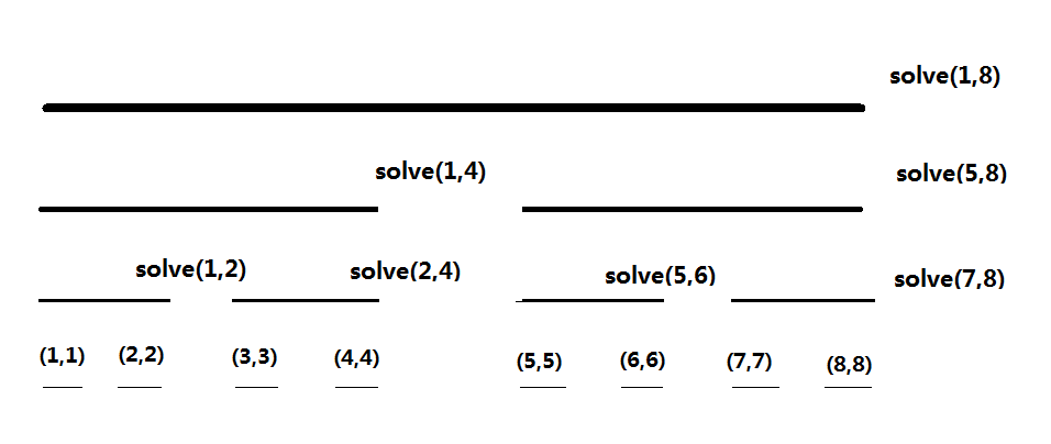
If we execute the algorithm flow described above, take point \(8\) as an example: its DP value is updated in the functions solve(1,8), solve(5,8), and solve(7,8). The three intervals used to update it are \((1,4)\), \((5,6)\), and \((7,7)\), which are disjoint. Similarly, for point \(5\), its DP value is resolved in solve(1,4), and the updating interval is \((1,4)\). Careful observation reveals that the DP value of a point \(i\) is updated \(\log\) times, and the intervals updating it are exactly the \(\log\) intervals into which \((1,i)\) is split on a segment tree. Thus, we indeed ensure that all valid \(j\) have updated point \(i\), satisfying condition 2.
Next, analyze the execution flow of our algorithm:
- The first function to finish is
solve(1,1). At this point, we find that \(dp_{1}\) has been computed. - The first function to execute the transition process is
solve(1,2). At this point, we find that \(dp_{2}\) has been updated. - The second function to finish is
solve(2,2). At this point, we find that \(dp_{2}\) has been computed. - Next,
solve(1,2)finishes, and the DP values for the interval \((1,2)\) are all computed. - The next function to execute the transition process is
solve(1,4). After this transition, we find that \(dp_{3}\) has been updated. - The next function to finish is
solve(3,3). We find that \(dp_{3}\) has been computed. - The next transition executed is
solve(2,4). At this point, \(dp_{4}\) was updated once by \((1,2)\) insolve(1,4)and again by \((3,3)\), so \(dp_{4}\) is also updated. solve(4,4)finishes, and \(dp_{4}\) is computed.solve(3,4)finishes, and the values for \((3,4)\) are computed.solve(1,4)finishes, and the values for \((1,4)\) are computed.- ……
By simulating the function flow, we observe that whenever solve(l,r) finishes, the DP values for the interval \((l,r)\) are fully computed. Since each time we execute the transition function, solve(l,mid) has already finished, every transition process we execute is valid, satisfying condition 1.
In the process above, we see that if we view the recursion tree of CDQ divide and conquer as a segment tree, then CDQ divide and conquer is the in-order traversal function of this segment tree. Thus, we process all DP values in order, only with the transition order split up, so the algorithm is correct.
Example Problems
SDOI2011 Intercept Missiles
A country has developed a missile interception system to defend against enemy missile attacks. However, this system has a flaw: although its first shot can reach any height and intercept missiles at any speed, each subsequent shot cannot exceed the height of the previous shot, and the speed of the intercepted missile cannot exceed that of the previous shot. One day, radar detects incoming enemy missiles. Since the system is still in the trial phase, only one set is available, so it may not intercept all missiles.
When not all missiles can be intercepted, we naturally choose the plan that minimizes national loss, i.e., intercepts the maximum number of missiles. However, there may be multiple optimal plans for intercepting the maximum number of missiles. If there are multiple optimal plans, we randomly select one as the final interception blueprint.
Our spies have obtained the heights and speeds of all enemy missiles. Your task is to calculate the probability that each missile is intercepted when executing the above decision.
Example Code
1 2 3 4 5 6 7 8 9 10 11 12 13 14 15 16 17 18 19 20 21 22 23 24 25 26 27 28 29 30 31 32 33 34 35 36 37 38 39 40 41 42 43 44 45 46 47 48 49 50 51 52 53 54 55 56 57 58 59 60 61 62 63 64 65 66 67 68 69 70 71 72 73 74 75 76 77 78 79 80 81 82 83 84 85 86 87 88 89 90 91 92 93 94 95 96 97 98 99 100 101 102 103 104 105 106 107 108 109 110 111 112 113 114 115 116 117 118 119 120 121 122 123 124 125 126 127 128 129 130 131 132 133 134 135 136 137 138 139 140 141 142 143 144 145 146 147 148 149 150 151 152 153 154 155 156 157 158 159 160 161 162 163 164 165 166 167 | |
Transforming Dynamic Problems into Static Problems
In the first two cases, the purpose of using CDQ divide and conquer is to recursively process point-pair relationships after halving the sequence to achieve good complexity. However, in this section, what is halved is not a general sequence but a time sequence.
This approach is suitable for some data structure problems that "require supporting xxx modifications and then xxx queries." Such problems have two characteristics:
- If the queries are offline, all operations naturally form a sequence in time order.
- Each modification is closely related to subsequent query operations. There will be \(O(n^2)\) such "modification-query" pairs.
We can use CDQ divide and conquer to partition this operation sequence and handle the relationships between modifications and queries.
Similar to CDQ divide and conquer for handling point-pair relationships, assume we are partitioning the sequence \((l,r)\). We first recursively handle the modification-query relationships between \((l,mid)\) and \((mid,r)\), then process all modification-query relationships where \(l \leq i \leq mid\) and \(mid+1 \leq j \leq r\), where \(i\) is a modification and \(j\) is a query.
Note that if the modifications are independent of each other, we do not need to handle the temporal order between \(l \leq i \leq mid\) and \(mid+1 \leq j \leq r\), or between solve(l,mid) and solve(mid+1,r) (e.g., ordinary addition/subtraction problems). However, if the modifications are not independent (e.g., assignment operations), the state of the sequence after a modification may depend on the previous sequence. In this case, the step of processing all modification-query relationships that cross \(mid\) must be placed between solve(l,mid) and solve(mid+1,r). The reason is the same as for CDQ divide and conquer optimizing 1D/1D dynamic programming: partitioning in in-order traversal ensures that each modification is executed strictly in time order.
Example Problems
Rectangle Addition and Rectangle Sum Query
Maintain a 2D array, supporting adding a number to a rectangular region and querying the sum of a rectangular region.
Solution Idea
For the non-modification version of this problem, i.e., "Given a 2D array, query the sum of a rectangular region multiple times," there is a classic approach using scanline with a segment tree. Specifically, each rectangle is split into insertion and deletion operations, each query is split into the difference of 2D prefix sums, and then processed offline. However, the original problem includes modifications, so this approach cannot be directly applied.
Try using CDQ divide and conquer. We offline all query and modification operations. These operations form a sequence with \(O(N^2)\) modification-query pairs. Following the general CDQ divide and conquer flow, we divide all relationships into three categories. In this layer of partitioning, we only handle modification-query relationships that cross \(mid\), and the remaining modification-query relationships are solved recursively.
We find that all modifications are completed before the queries. At this point, the original problem is equivalent to "There are static rectangles on the plane, and we continuously query the sum of a rectangular region."
Use a scanline to handle all modification-query relationships crossing \(mid\) in \(O(n\log n)\) time. The remaining task is to recursively partition the modification-query relationships on the left and right sides.
In this CDQ divide and conquer implementation, each query is processed \(O(\log n)\) times. However, this is fine because the modifications contributing to this query are disjoint each time. The overall time complexity is \(T(n)=T(\lfloor \frac{n}{2} \rfloor)+T(\lceil \frac{n}{2} \rceil)+ O(n\log n)=O(n\log^2n)\).
Observing the algorithm flow, we see that initially we could only solve the static rectangle addition and sum query problem. However, by simply using CDQ divide and conquer, we can offline solve a dynamic rectangle addition and sum query problem. The essence of transforming dynamic problems into static problems lies in CDQ divide and conquer processing only the modification-query relationships crossing a certain point each time. This way, we only need to consider the simple problem of "all queries occur after modifications." It is precisely because of this that CDQ divide and conquer is called a "tool for transforming dynamic problems into static problems."
[Ynoi2016] Insects in the Mirror
Maintain a sequence \(a_i\) of length \(n\), with \(m\) operations.
- Change the value of the interval \([l,r]\) to \(x\);
- Query how many distinct numbers appear in the interval \([l,r]\), i.e., multiple occurrences of the same number count as one.
In one sentence: interval assignment and interval color counting.
Solution Idea
Maintain the position of the first same-colored point to the left of each position, denoted as \(pre_{i}\). Then interval color counting is transformed into a classic 2D point counting problem.
By treating consecutive segments of the same color as a single point, it can be proven that the total change in \(pre\) is \(O(n+m)\), i.e., each operation only causes \(O(1)\) changes in \(pre\) values. Thus, we can use CDQ divide and conquer to solve the dynamic single-point addition and rectangle sum query problem.
The specific changes in the \(pre\) array can be handled using std::set. This technique of using set to maintain consecutive intervals is also known as old driver tree.
Example Code
1 2 3 4 5 6 7 8 9 10 11 12 13 14 15 16 17 18 19 20 21 22 23 24 25 26 27 28 29 30 31 32 33 34 35 36 37 38 39 40 41 42 43 44 45 46 47 48 49 50 51 52 53 54 55 56 57 58 59 60 61 62 63 64 65 66 67 68 69 70 71 72 73 74 75 76 77 78 79 80 81 82 83 84 85 86 87 88 89 90 91 92 93 94 95 96 97 98 99 100 101 102 103 104 105 106 107 108 109 110 111 112 113 114 115 116 117 118 119 120 121 122 123 124 125 126 127 128 129 130 131 132 133 134 135 136 137 138 139 140 141 142 143 144 145 146 147 148 149 150 151 152 153 154 155 156 157 158 159 160 161 162 163 164 165 166 167 168 169 170 171 172 173 174 175 176 177 178 179 180 181 182 183 184 185 186 187 188 189 190 191 192 193 194 195 196 197 198 199 200 201 202 203 204 205 206 207 208 209 210 211 212 213 214 215 216 217 218 219 220 221 222 223 224 225 226 227 228 229 230 231 232 233 234 235 236 237 238 239 240 241 | |
[HNOI2010] City Construction
PS Country is a large country with many cities. King Louis has racked his brains for urban transportation construction. Louis can build roads between certain cities, with different costs for building roads between different cities.
Louis hopes to build the minimum number of roads to connect all cities. However, due to certain factors, the cost of building roads between cities changes over time. Louis continuously receives messages about changes in road construction costs. He wants to know the minimum total cost to connect the cities immediately after each message. Louis decides to ask for your help to complete this task.
In one sentence: Given a graph supporting dynamic modifications of edge weights, output the minimum cost of the minimum spanning tree after each edge weight modification.
Solution Idea
In fact, there is an approach using segment tree divide and conquer with LCT to solve this problem, but this implementation has a large constant and may require sophisticated constant optimization to pass. Therefore, consider using CDQ divide and conquer to solve this problem.
Unlike problems typically solved by CDQ divide and conquer, there is no modification-query relationship to partition here because we cannot separately consider "the contribution of modifying an edge to the entire graph's minimum spanning tree." The traditional CDQ divide and conquer approach does not seem to work well.
From the previous example, we see that general CDQ divide and conquer has a special connection with segment trees: during CDQ divide and conquer, we implicitly build a segment tree (because the recursion tree of CDQ divide and conquer is a segment tree). Usually, CDQ considers the relationship between left and right children of the segment tree. For this problem, we need to consider the relationship between parent and child; in other words, when processing the interval $solve(l,r)$, if we can reduce the graph's scale to a variable related to the interval length, we can solve the problem.
So how do we design the algorithm specifically?
Suppose we are constructing the edge set of the minimum spanning tree for the interval \((l,r)\), and we know the edge set of its parent's minimum spanning tree. We assign edge weights of \(+ \infty\) and \(-\infty\) to the edges that change in the interval \((l,r)\), respectively, and run Kruskal once for each to find the edges that appear in the minimum spanning tree.
For an edge:
- If all modified edge weights in the minimum spanning tree are assigned \(+\infty\), and this edge does not appear in the tree, then it cannot appear in the minimum spanning tree for the queries in \((l,r)\). Thus, we only add the tree edges of the minimum spanning tree to the edge set for \((l,r)\).
- If all modified edge weights in the minimum spanning tree are assigned \(-\infty\), and this edge appears in the tree, then it must appear in the minimum spanning tree for the interval \((l,r)\). In this case, we can use a union-find set to contract the points connected by these edges and add the edge weights to the answer.
This way, we construct the edge set for the interval \((l,r)\). The minimum spanning tree computed with these edges is equivalent to directly computing the original graph's minimum spanning tree.
So why is our complexity correct?
First, modified edges are always added to our edge set, and the number of such edges is \(O(len)\).
Next, we need to prove that there are not too many unmodified edges in the edge set. We only add tree edges from the minimum spanning tree with all edge weights set to \(+\infty\), so the number of edges we add does not exceed the number of vertices in the current graph.
Now we only need to prove that the number of vertices per recursion level is \(O(len)\) to show that the number of edges is \(O(len)\).
Proving that the number of vertices is \(O(len)\) becomes straightforward. Each time we recursively descend, we contract edges that are unmodified edges appearing in the \(-\infty\) spanning tree. Conversely, we cut all modified edges that appear in the \(-\infty\) spanning tree. Clearly, we cut at most \(len\) edges, so the graph splits into at most \(O(len)\) connected components, meaning the new graph has \(O(len)\) vertices. Thus, we prove that the graph we run Kruskal on each time is \(O(len)\) in size, so the time complexity per level is \(O(n\log n)\).
The overall time complexity is \(T(n)=T(\lfloor \frac{n}{2} \rfloor)+T(\lceil \frac{n}{2} \rceil)+ O(n\log n)=O(n\log^2n)\).
The code implementation may be somewhat challenging. Note that the union-find set cannot use path compression, as it would not support rollback operations. Also, when performing contraction operations, there is no need to actually contract; instead, each level's Kruskal can be directly performed on the previous level's union-find set.
Example Code
1 2 3 4 5 6 7 8 9 10 11 12 13 14 15 16 17 18 19 20 21 22 23 24 25 26 27 28 29 30 31 32 33 34 35 36 37 38 39 40 41 42 43 44 45 46 47 48 49 50 51 52 53 54 55 56 57 58 59 60 61 62 63 64 65 66 67 68 69 70 71 72 73 74 75 76 77 78 79 80 81 82 83 84 85 86 87 88 89 90 91 92 93 94 95 96 97 98 99 100 101 102 103 104 105 106 107 108 109 110 111 112 113 114 115 116 117 118 119 120 121 122 123 124 125 126 127 128 129 130 131 132 133 134 135 136 137 138 139 140 141 142 143 144 145 146 147 148 149 150 151 152 153 154 155 156 157 158 159 160 161 162 163 164 165 166 167 168 169 170 171 172 173 174 175 176 177 178 179 180 181 182 183 184 185 186 187 188 189 190 191 192 193 194 195 196 197 198 199 200 201 202 203 204 205 206 207 208 209 210 211 212 213 214 215 216 217 218 219 220 221 222 223 224 225 226 227 | |
References and Notes
本页面最近更新:,更新历史
发现错误?想一起完善? 在 GitHub 上编辑此页!
本页面贡献者:OI-wiki
本页面的全部内容在 CC BY-SA 4.0 和 SATA 协议之条款下提供,附加条款亦可能应用