Fenwick Tree
Introduction
A Fenwick Tree (Binary Indexed Tree) is a data structure that supports single-point modification and interval query with small code size.
What are 'single-point modification' and 'interval query'?
Consider the following problem:
Given a sequence \(a\), you need to perform two types of operations:
- Given \(x, y\), increment \(a[x]\) by \(y\).
- Given \(l, r\), compute the sum of \(a[l \ldots r]\).
Here, the first operation is "single-point modification", and the second is "interval query".
Similarly, there are: "interval modification" and "single-point query". Examples:
- Interval modification: given \(l, r, x\), increment each number in \(a[l \ldots r]\) by \(x\);
- Single-point query: given \(x\), compute the value of \(a[x]\).
Note that interval problems are generally strictly stronger than single-point problems, because operating on a single point is equivalent to operating on an interval of length \(1\).
The information and operations maintained by a standard Fenwick Tree must satisfy associativity and invertibility (i.e., the operation must be reversible), such as addition (sum), multiplication (product), XOR, etc.
- Associativity: \((x \circ y) \circ z = x \circ (y \circ z)\), where \(\circ\) is a binary operator.
- Invertibility: The operation has an inverse, meaning given \(x \circ y\) and \(x\), we can compute \(y\).
Note:
- Multiplication under modulo requires each element to have an inverse to be invertible (which exists when the modulus is prime);
- For example, \(\gcd\), \(\max\) are not invertible, so they cannot be handled by a standard Fenwick Tree. However:
- Two Fenwick Trees can be used to handle range minimum queries, see Efficient Range Minimum Queries using Binary Indexed Trees.
- This page will also introduce an extended Fenwick Tree that supports non-invertible information queries with \(\Theta(\log^2n)\) time complexity.
In fact, the problems solvable by a Fenwick Tree are a subset of those solvable by a Segment Tree: anything a Fenwick Tree can do, a Segment Tree can also do; but not vice versa. However, the Fenwick Tree has much shorter code and smaller constant factors, making it still worth learning.
Sometimes, with the help of difference arrays and auxiliary arrays, a Fenwick Tree can also solve stronger problems like interval addition with single-point query and interval addition with interval sum.
Fenwick Tree
First Impression
Let's start with an example: we want to know the prefix sum of \(a[1 \ldots 7]\). How?
One approach: \(a_1 + a_2 + a_3 + a_4 + a_5 + a_6 + a_7\), requiring summing 7 numbers.
But if we know three numbers \(A\), \(B\), \(C\), where \(A\) is the sum of \(a[1 \ldots 4]\), \(B\) is the sum of \(a[5 \ldots 6]\), and \(C\) is the sum of \(a[7 \ldots 7]\) (which is just \(a[7]\)). How would you compute it? You'd answer: \(A + B + C\), requiring only 3 sums.
This is why the Fenwick Tree can quickly compute information: we can always split a prefix \([1, n]\) into at most \(\boldsymbol{\log n}\) intervals such that the information of these \(\log n\) intervals is known.
Thus, we only need to merge the information of these \(\log n\) intervals to get the answer. Compared to directly merging \(n\) pieces of information, efficiency is greatly improved.
Clearly, the information must satisfy associativity; otherwise, such merging is not possible.
The following diagram illustrates how a Fenwick Tree works:
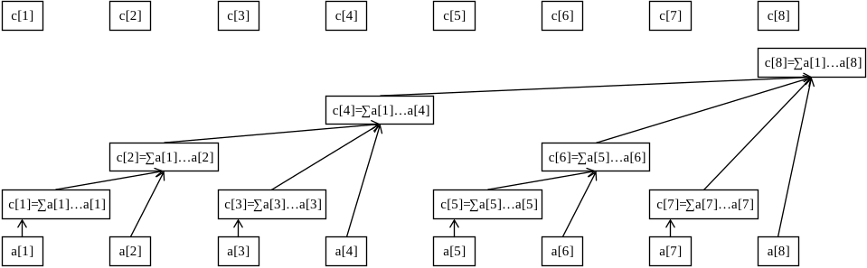
The bottom eight squares represent the original data array \(a\). The uneven squares above (which are the same as the top eight squares) represent the \(c\) array, which is the "superior" of \(a\).
The \(c\) array stores the sum of certain intervals of \(a\). In other words, the information of these intervals is known, and our goal is to split the query prefix into these small intervals.
For example, from the diagram:
- \(c_2\) manages \(a[1 \ldots 2]\);
- \(c_4\) manages \(a[1 \ldots 4]\);
- \(c_6\) manages \(a[5 \ldots 6]\);
- \(c_8\) manages \(a[1 \ldots 8]\);
- The remaining \(c[x]\) each manage only \(a[x]\) itself (can be seen as a length-1 interval \(a[x \ldots x]\)).
We can see that \(c[x]\) always manages an interval whose right endpoint is \(x\). For now, we don't care about the left endpoint; let's first see how queries work.
Example: compute the sum of \(a[1 \ldots 7]\).
Process: Start from \(c_{7}\) and jump forward. Find that \(c_{7}\) only manages \(a_{7}\); then go to \(c_{6}\), which manages \(a[5 \ldots 6]\); then jump to \(c_{4}\), which manages \(a[1 \ldots 4]\); then try to jump to \(c_0\), but \(c_0\) doesn't exist, so stop.
The \(c\) we found are \(c_7, c_6, c_4\). These are exactly the three small intervals that \(a[1 \ldots 7]\) splits into. Merging them gives the answer: \(c_7 + c_6 + c_4\).
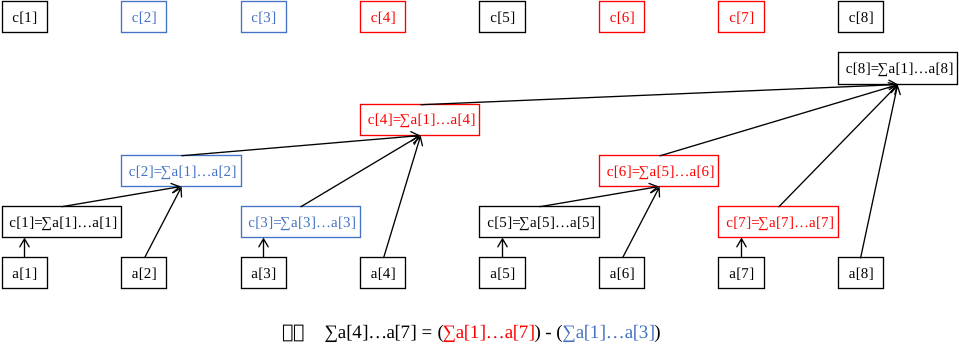
Example: compute the sum of \(a[4 \ldots 7]\).
We start from \(c_7\), jump to \(c_6\), then to \(c_4\). Now we see it manages the sum of \(a[1 \ldots 4]\), but we don't want the part \(a[1 \ldots 3]\). What to do? Simply subtract the sum of \(a[1 \ldots 3]\).
So consider transforming the query for \(a[4 \ldots 7]\) into querying the sum of \(a[1 \ldots 7]\) and the sum of \(a[1 \ldots 3]\), then taking their difference.
Managed Interval
Now the question: how far to the left does \(c[x](x \ge 1)\) manage? That is, what is the interval length?
In a Fenwick Tree, \(c[x]\) manages an interval of length \(2^{k}\), where:
- Let the least significant bit be bit 0. Then \(k\) is exactly the position of the lowest
1in the binary representation of \(x\); - \(2^k\) (the length of \(c[x]\)'s managed interval) is exactly the number formed by the lowest
1and all trailing0s in \(x\)'s binary representation.
For example, which interval does \(c_{88}\) manage?
Since \(88_{(10)}=01011000_{(2)}\), the binary formed by the lowest 1 and trailing 0s is 1000, i.e., \(8\), so \(c_{88}\) manages 8 elements of \(a\).
Thus, \(c_{88}\) represents the interval information of \(a[81 \ldots 88]\).
Let \(\operatorname{lowbit}(x)\) denote the number formed by the lowest 1 and all trailing 0s in \(x\). Then \(c[x]\) manages the interval \([x-\operatorname{lowbit}(x)+1, x]\).
Note
\(\operatorname{lowbit}\) does not refer to the position \(k\) of the lowest 1, but to the number \(2^k\) formed by that 1 and all trailing 0s.
How to compute lowbit? From bitwise operations: lowbit(x) = x & -x.
Principle of lowbit
Inverting all bits of x and adding 1 gives the binary encoding of -x. For example, the binary of \(6\) is 110, invert to get 001, add 1 to get 010.
Suppose the original binary of x is (...)10...00. After inversion, we get [...]01...11. Adding 1 gives [...]10...00, which is the binary of -x. Here, the first 1 in x is the lowest 1.
The (...) and [...] parts have opposite bits, so x & -x = (...)10...00 & [...]10...00 = 10...00, which is exactly lowbit.
Implementation
1 2 3 4 5 6 7 8 | |
1 2 3 4 5 6 7 8 9 | |
Interval Query
Now let's look at the specific operations of the Fenwick Tree, starting with interval queries.
Recall the process of querying \(a[4 \ldots 7]\): we transformed it into two sub-queries: query the sum of \(a[1 \ldots 7]\) and query the sum of \(a[1 \ldots 3]\), then took the difference.
In fact, any interval query can be done this way: querying the sum of \(a[l \ldots r]\) is the sum of \(a[1 \ldots r]\) minus the sum of \(a[1 \ldots l - 1]\), thus transforming an interval problem into a prefix problem, which is easier to handle.
Indeed, transforming interval queries about \(l \ldots r\) into prefix queries about \(1 \ldots r\) and \(1 \ldots l - 1\) and then taking the difference is a very common technique in competitive programming.
How to do prefix queries? Recall querying \(a[1 \ldots 7]\):
Start from \(c_{7}\), jump forward, find \(c_{7}\) only manages \(a_{7}\); then go to \(c_{6}\), which manages \(a[5 \ldots 6]\); then jump to \(c_{4}\), which manages \(a[1 \ldots 4]\); then try to jump to \(c_0\), but \(c_0\) doesn't exist, stop.
The \(c\) we found are \(c_7, c_6, c_4\), which are exactly the three small intervals \(a[1 \ldots 7]\) splits into. Merging gives \(c_7 + c_6 + c_4\).
Observing the process, each forward jump must go to the position one left of the current interval's left endpoint, as the new interval's right endpoint, to ensure the prefix is split without overlap or omission. For example, \(c_6\) manages \(a[5 \ldots 6]\), next jump to \(5 - 1 = 4\), i.e., visit \(c_4\).
We can describe the process of querying \(a[1 \ldots x]\):
- Start from \(c[x]\), which manages \(a[x-\operatorname{lowbit}(x)+1 \ldots x]\);
- Set \(x \gets x - \operatorname{lowbit}(x)\). If \(x = 0\), we've reached the end, stop; otherwise go back to step 1.
- Merge the \(c\) encountered during jumps.
In implementation, we don't need to collect all \(c\) first and then merge; we can merge while jumping.
For example, if we maintain sum, set initial \(\mathrm{ans} = 0\), then for each \(c[x]\) encountered, do \(\mathrm{ans} \gets \mathrm{ans} + c[x]\). Finally, \(\mathrm{ans}\) is the merged result.
Implementation
1 2 3 4 5 6 7 8 | |
1 2 3 4 5 6 | |
Fenwick Tree and Its Tree Structure Properties
Before explaining single-point modification, let's discuss some basic properties of the Fenwick Tree and its tree structure, which helps better understand single-point modification.
We define:
- \(l(x) = x - \operatorname{lowbit}(x) + 1\). That is, \(l(x)\) is the left endpoint of \(c[x]\)'s managed range.
- For any positive integer \(x\), we can always express \(x\) as \(s \times 2^{k + 1} + 2^k\), where \(\operatorname{lowbit}(x) = 2^k\).
- Below, "\(c[x]\) and \(c[y]\) are disjoint" means the managed ranges of \(c[x]\) and \(c[y]\) do not intersect, i.e., \([l(x), x]\) and \([l(y), y]\) are disjoint. Similarly for "\(c[x]\) is contained in \(c[y]\)".
Property \(\boldsymbol{1}\): For \(\boldsymbol{x \le y}\), either \(\boldsymbol{c[x]}\) and \(\boldsymbol{c[y]}\) are disjoint, or \(\boldsymbol{c[x]}\) is contained in \(\boldsymbol{c[y]}\).
Proof
Proof: Suppose \(c[x]\) and \(c[y]\) intersect, i.e., \([l(x), x]\) and \([l(y), y]\) intersect, then \(l(y) \le x \le y\).
Write \(y\) as \(s \times 2^{k +1} + 2^k\), then \(l(y) = s \times 2^{k + 1} + 1\). So \(x\) can be written as \(s \times 2^{k +1} + b\), where \(1 \le b \le 2^k\).
Note \(\operatorname{lowbit}(x) = \operatorname{lowbit}(b)\). Since \(b - \operatorname{lowbit}(b) \ge 0\),
\(l(x) = x - \operatorname{lowbit}(x) + 1 = s \times 2^{k +1} + b - \operatorname{lowbit}(b) +1 \ge s \times 2^{k +1} + 1 = l(y)\), i.e., \(l(y) \le l(x) \le x \le y\).
So if \(c[x]\) and \(c[y]\) intersect, then \(c[x]\)'s range is completely contained in \(c[y]\).
Property \(\boldsymbol{2}\): \(\boldsymbol{c[x]}\) is strictly contained in \(\boldsymbol{c[x + \operatorname{lowbit}(x)]}\).
Proof
Proof: Let \(y = x + \operatorname{lowbit}(x)\), \(x = s \times 2^{k + 1} + 2^k\), then \(y = (s + 1) \times 2^{k +1}\), \(l(x) = s \times 2^{k + 1} + 1\).
Note \(\operatorname{lowbit}(y) \ge 2^{k + 1}\), so \(l(y) = (s + 1) \times 2^{k + 1} - \operatorname{lowbit}(y) + 1 \le s \times 2^{k +1} + 1= l(x)\), i.e., \(l(y) \le l(x) \le x < y\).
So \(c[x]\) is strictly contained in \(c[x + \operatorname{lowbit}(x)]\).
Property \(3\): For any \(\boldsymbol{x < y < x + \operatorname{lowbit}(x)}\), \(\boldsymbol{c[x]}\) and \(\boldsymbol{c[y]}\) are disjoint.
Proof
Proof: Let \(x = s \times 2^{k + 1} + 2^k\), then \(y = x + b = s \times 2^{k + 1} + 2^k + b\), where \(1 \le b < 2^k\).
Note \(\operatorname{lowbit}(y) = \operatorname{lowbit}(b)\). Since \(b - \operatorname{lowbit}(b) \ge 0\),
\(l(y) = y - \operatorname{lowbit}(y) + 1 = x + b - \operatorname{lowbit}(b) + 1 > x\), i.e., \(l(x) \le x < l(y) \le y\).
So \(c[x]\) and \(c[y]\) are disjoint.
With these three properties, let's look at the tree structure of the Fenwick Tree (ignore edges from \(a\) to \(c\)).
In fact, the tree structure of the Fenwick Tree is obtained by connecting \(x\) to \(x + \operatorname{lowbit}(x)\), where \(x + \operatorname{lowbit}(x)\) is the parent of \(x\).
Note: when considering the tree structure, we ignore the size limit of the Fenwick Tree, i.e., we consider an infinite tree for analysis. In practice, we only use \(c[x]\) for \(x \le n\), where \(n\) is the original array length.
This tree naturally has many nice properties. Here are some (let \(fa[u]\) denote the direct parent of \(u\)):
- \(u < fa[u]\).
- \(u\) is greater than any descendant of \(u\) and less than any ancestor of \(u\).
- The \(\operatorname{lowbit}\) of \(u\) is strictly less than the \(\operatorname{lowbit}\) of \(fa[u]\).
Proof
Let \(y = x + \operatorname{lowbit}(x)\), \(x = s \times 2^{k + 1} + 2^k\), then \(y = (s + 1) \times 2^{k +1}\). Note \(\operatorname{lowbit}(y) \ge 2^{k + 1} > \operatorname{lowbit}(x)\), proved.
- The height of node \(x\) is \(\log_2\operatorname{lowbit}(x)\), i.e., the position of the lowest
1in \(x\)'s binary.
Definition of height
The height \(h(x)\) of node \(x\) satisfies: if \(x \bmod 2 = 1\), then \(h(x) = 0\); otherwise \(h(x) = \max(h(y)) + 1\), where \(y\) ranges over all children of \(x\) (here \(x\) has at least one child \(x - 1\)).
That is, a node's height is exactly one more than the height of its tallest child. If a node has no children, its height is \(0\).
Height is introduced here to explain complexity later.
- \(c[u]\) is strictly contained in \(c[fa[u]]\) (Property 2).
- \(c[u]\) is strictly contained in \(c[v]\), where \(v\) is any ancestor of \(u\) (induction from previous property).
- \(c[u]\) strictly contains \(c[v]\), where \(v\) is any descendant of \(u\) (reverse of above).
- For any \(v' > u\), if \(v'\) is not an ancestor of \(u\), then \(c[u]\) and \(c[v']\) are disjoint.
Proof
Among \(u\) and its ancestors, there must be a node \(v\) such that \(v < v' < fa[v]\). By Property 3, \(c[v']\) is disjoint from \(c[v]\), and \(c[v]\) contains \(c[u]\), so \(c[v']\) is disjoint from \(c[u]\).
- For any \(v < u\), if \(v\) is not in the subtree of \(u\), then \(c[u]\) and \(c[v]\) are disjoint (reverse of above).
- For any \(v > u\), \(c[u]\) is strictly contained in \(c[v]\) if and only if \(v\) is an ancestor of \(u\) (summary of above). This is the core principle of single-point modification in Fenwick Tree.
- Let \(u = s \times 2^{k + 1} + 2^k\), then the number of its children is \(k = \log_2\operatorname{lowbit}(u)\), with indices \(u - 2^t(0 \le t < k)\).
- Example: suppose \(k = 3\), \(u\)'s binary is
...1000, then \(u\) has three children, with binaries...0111,...0110,...0100.
- Example: suppose \(k = 3\), \(u\)'s binary is
Proof
Subtracting \(2^t\) from a number \(x\) flips the \(t\)-th bit of \(x\), while lower bits remain unchanged.
Consider a child \(v\) of \(u\), with \(v + \operatorname{lowbit}(v) = u\), i.e., \(v = u - 2^t\) and \(\operatorname{lowbit}(v) = 2^t\). Let \(u = s \times 2^{k + 1} + 2^k\).
For \(\boldsymbol{0 \le t < k}\): the \(t\)-th bit and beyond of \(u\) are \(0\), so \(v = u - 2^t\) has its \(t\)-th bit become \(1\), and trailing bits still \(0\), satisfying \(\operatorname{lowbit}(v) = 2^t\).
For \(\boldsymbol{t = k}\): \(v = u - 2^k\), the \(k\)-th bit of \(v\) becomes \(0\), not satisfying \(\operatorname{lowbit}(v) = 2^t\).
For \(\boldsymbol{t > k}\): \(v = u - 2^t\), the \(k\)-th bit of \(v\) is \(1\), so \(\operatorname{lowbit}(v) = 2^k\), not satisfying \(\operatorname{lowbit}(v) = 2^t\).
- The managed intervals of \(u\)'s children exactly concatenate to \([l(u), u - 1]\).
- Example: suppose \(k = 3\), \(u\)'s binary is
...1000, then \(u\) has three children:...0111,...0110,...0100. c[...0100]representsa[...0001 ~ ...0100].c[...0110]representsa[...0101 ~ ...0110].c[...0111]representsa[...0111 ~ ...0111].- The union of these three intervals is exactly
a[...0001 ~ ...0111], i.e., \([l(u), u - 1]\).
- Example: suppose \(k = 3\), \(u\)'s binary is
Proof
\(u\)'s children can be expressed as \(u - 2^t(0 \le t < k)\). Note that smaller \(t\) gives larger \(u - 2^t\), representing intervals more to the right. Let \(f(t) = u - 2^t\), then \(f(k - 1), f(k - 2), \ldots, f(0)\) are \(u\)'s children from left to right.
Note \(\operatorname{lowbit}(f(t)) = 2^t\), so \(l(f(t)) = u - 2^t - 2^t + 1 = u - 2^{t + 1} + 1\).
Consider two adjacent children \(f(t + 1)\) and \(f(t)\). The right endpoint of the former's interval is \(f(t + 1) = u - 2^{t + 1}\), and the left endpoint of the latter's interval is \(l(f(t)) = u - 2^{t + 1} + 1\), exactly adjacent.
Consider the leftmost child \(f(k - 1)\): its left boundary \(l(f(k - 1)) = u - 2^k + 1\) is exactly \(l(u)\).
Consider the rightmost child \(f(0)\): its right boundary is \(u - 1\).
Thus, the children's intervals exactly concatenate to \([l(u), u - 1]\).
Single-Point Modification
Now consider how to modify a single point \(a[x]\).
Our goal is to quickly and correctly maintain the \(c\) array. For efficiency, we only need to traverse and modify all \(c[y]\) that manage \(a[x]\), because other \(c\) clearly remain unchanged.
Any \(c[y]\) managing \(a[x]\) must contain \(c[x]\) (by Property 1), so \(y\) is an ancestor of \(x\) in the tree structure. Therefore, we start from \(x\) and repeatedly jump to the parent until we exceed the original array length.
Let \(n\) be the size of \(a\). The process for single-point modification of \(a[x]\) is:
- Initially set \(x' = x\).
- Modify \(c[x']\).
- Set \(x' \gets x' + \operatorname{lowbit}(x')\). If \(x' > n\), we've reached the end, stop; otherwise go back to step 2.
The type of interval information and single-point modification determines how \(c[x']\) is modified. Examples:
- If \(c[x']\) maintains interval sum, and the modification is to add \(p\) to \(a[x]\), then modify all \(c[x']\) by adding \(p\).
- If \(c[x']\) maintains interval product, and the modification is to multiply \(a[x]\) by \(p\), then modify all \(c[x']\) by multiplying by \(p\).
However, the flexibility of single-point modification means the modification type and maintained information may not be the same operation. For example, if \(c[x']\) maintains interval sum and we want to set \(a[x]\) to \(p\), we can transform it to adding \(p - a[x]\) to \(a[x]\). If we want to multiply \(a[x]\) by \(p\), transform to adding \(a[x] \times p - a[x]\).
Below is an implementation for maintaining interval sum with single-point addition.
Implementation
1 2 3 4 5 6 | |
1 2 3 4 | |
Building the Tree
That is, given an initial sequence, build the Fenwick Tree (preprocess all \(c\)).
Usually, we can directly treat it as \(n\) single-point modifications, with time complexity \(\Theta(n \log n)\) (complexity analysis later).
For example, given sequence \(a = (5, 1, 4)\), build the tree by treating it as adding \(5\) to \(a[1]\), adding \(1\) to \(a[2]\), and adding \(4\) to \(a[3]\).
There is also a \(\Theta(n)\) building method, see the \(\Theta(n)\) Building section.
Complexity Analysis
Space complexity is clearly \(\Theta(n)\).
Time complexity:
- For interval query: the iteration \(x \gets x - \operatorname{lowbit}(x)\) can be seen as gradually changing all
1s in \(x\)'s binary from low to high to0. The number of split intervals equals the number of1s in \(x\) (i.e., \(\operatorname{popcount}(x)\)). Thus, single query time is \(\Theta(\log n)\); - For single-point modification: when jumping to parents, the height strictly increases, and we always have \(x \le n\). Since the height of node \(x\) is \(\log_2\operatorname{lowbit}(x)\), the height jumped to won't exceed \(\log_2n\), so the number of \(c\) accessed is \(\Theta(\log n)\). Thus, single modification time is \(\Theta(\log n)\).
Interval Addition and Interval Sum
Prerequisite: Prefix Sum & Difference.
This problem can be solved using two Fenwick Trees maintaining a difference array.
Consider the difference array \(d\) of sequence \(a\), where \(d[i] = a[i] - a[i - 1]\). Since the prefix sum of the difference array is the original array, \(a_i=\sum_{j=1}^i d_j\).
Similarly, we transform interval sum queries into prefix sum queries via difference. Consider querying the sum of \(a[1 \ldots r]\), i.e., \(\sum_{i=1}^{r} a_i\):
Observing this, each \(d_j\) is added \(r - j + 1\) times. Continue:
\(\sum_{i=1}^r d_i\) does not give \(\sum_{i=1}^r d_i \times i\), so we need two Fenwick Trees to maintain the sums of \(d_i\) and \(d_i \times i\).
How to do interval addition? Consider adding \(x\) to \(a[l \ldots r]\) and its effect on \(d\).
Since \(d[i] = a[i] - a[i - 1]\),
- \(a[l]\) increases by \(v\) while \(a[l - 1]\) unchanged, so \(d[l]\) increases by \(v\).
- \(a[r + 1]\) unchanged while \(a[r]\) increases by \(v\), so \(d[r + 1]\) decreases by \(v\).
- For any \(i\) not equal to \(l\) or \(r+1\), either both \(a[i]\) and \(a[i - 1]\) change or both don't. \(a[i] + v - (a[i - 1] + v) = a[i] - a[i - 1]\), so other \(d[i]\) remain unchanged.
Thus, the maintenance method: for the Fenwick Tree maintaining \(d_i\), add \(v\) at \(l\) and \(-v\) at \(r + 1\); for the Fenwick Tree maintaining \(d_i \times i\), add \(v \times l\) at \(l\) and \(-v \times (r + 1)\) at \(r + 1\).
The weaker problem, "interval addition with single-point query", only needs one Fenwick Tree maintaining \(d_i\). To query \(a[x]\), compute the sum of \(d[1 \ldots x]\).
Here is the code for "interval addition and interval sum":
Implementation
1 2 3 4 5 6 7 8 9 10 11 12 13 14 15 16 17 18 19 20 21 22 23 24 25 26 27 28 29 30 | |
1 2 3 4 5 6 7 8 9 10 11 12 13 14 15 16 17 18 19 20 21 22 23 24 25 26 27 28 29 30 31 32 33 34 35 36 | |
Based on this principle, we can implement "interval multiplication and interval product", "interval XOR with a number, query interval XOR", etc., as long as the maintained information and interval operation are the same operation. Interested readers can try.
2D Fenwick Tree
Single-Point Modification, Submatrix Query
A 2D Fenwick Tree, also called Fenwick Tree of Fenwick Trees, maintains single-point modification and prefix information on a 2D array.
Similar to 1D, let \(c(x, y)\) represent the total information of the matrix from \(a(x - \operatorname{lowbit}(x) + 1, y - \operatorname{lowbit}(y) + 1)\) to \(a(x, y)\), i.e., a matrix with bottom-right corner \(a(x, y)\), height \(\operatorname{lowbit}(x)\), width \(\operatorname{lowbit}(y)\).
For single-point modification, define:
That is, \(f(x, i)\) is the \(i\)-th level ancestor of \(x\) in the tree structure (0-th ancestor is itself).
Then only \(c(f(x, i), f(y, j))\) manage \(a(x, y)\). When modifying \(a(x, y)\), modify all \(c(f(x, i), f(y, j))\) where \(f(x, i) \le n\), \(f(y, j) \le m\).
Proof of correctness
\(c(p, q)\) manages \(a(x, y)\). Find ranges for \(p\) and \(q\).
Consider a 1D Fenwick Tree \(c_1\) of size \(n\) (corresponding to \(a_1\)) and a 1D Fenwick Tree \(c_2\) of size \(m\) (corresponding to \(a_2\)).
The proposition is equivalent to: conditions for \(c_1(p)\) managing \(a_1[x]\) and \(c_2(q)\) managing \(a_2[y]\).
That is, in the tree structure, \(p\) is \(x\) or an ancestor
本页面最近更新:,更新历史
发现错误?想一起完善? 在 GitHub 上编辑此页!
本页面贡献者:OI-wiki
本页面的全部内容在 CC BY-SA 4.0 和 SATA 协议之条款下提供,附加条款亦可能应用