Tree Basics

Introduction

The tree in graph theory looks like a real-life tree, but we usually consider it with the root placed at the top when solving problems. This data structure resembles an upside-down tree, hence the name.

Definition

A tree without a fixed root node is called an unrooted tree. Unrooted trees have several equivalent formal definitions:

• A connected undirected graph with \(n\) vertices and \(n-1\) edges.
• A connected undirected graph without cycles.
• An undirected graph in which there is exactly one simple path between any two vertices.
• A connected graph in which every edge is a bridge.
• A graph without cycles, such that adding any edge between two distinct vertices results in a graph containing exactly one cycle.

Based on an unrooted tree, designating a vertex as the root forms a rooted tree. Rooted trees are often still represented as undirected graphs, but with a defined hierarchical relationship between vertices, as detailed below.

Definitions Related to Trees

Applicable to Both Unrooted and Rooted Trees

• Forest: A graph where each connected component is a tree. By definition, a single tree is also a forest.
• Spanning tree: A spanning subgraph of a connected undirected graph that is also a tree. That is, selecting \(n - 1\) edges from the graph's edge set to connect all vertices.

• Leaf node of an unrooted tree: A vertex with degree at most \(1\).

  Why not exactly degree \(1\)?

  Consider the case \(n = 1\).

• Leaf node of a rooted tree: A vertex with no children.

Applicable Only to Rooted Trees

• Parent node: For every vertex except the root, defined as the second vertex on the path from that vertex to the root. The root has no parent.
• Ancestor: All vertices on the path from a vertex to the root, excluding the vertex itself. The set of ancestors of the root is empty.
• Child node: If \(u\) is the parent of \(v\), then \(v\) is a child of \(u\). The order of children is generally not distinguished, except in binary trees.
• Depth of a vertex: The number of edges on the path to the root.
• Height of a tree: The maximum depth among all vertices.
• Siblings: Multiple children of the same parent are siblings.
• Descendant: The children of a vertex and their descendants. Alternatively, if \(u\) is an ancestor of \(v\), then \(v\) is a descendant of \(u\).

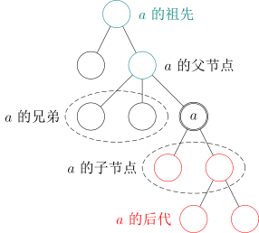
• Subtree: The subgraph containing a vertex after removing the edge connecting it to its parent.

  

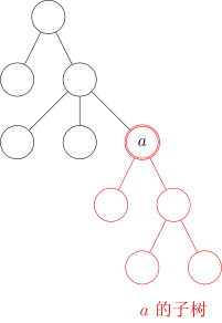
Special Types of Trees

• Chain/Path graph: A tree where no vertex is connected to more than \(2\) edges.
• Star: A tree where there exists a vertex \(u\) such that all other vertices are connected to \(u\).
• Rooted binary tree: A rooted tree where each vertex has at most two children. Often, the order of the two children is distinguished, called the left child and the right child. In most contexts, the term binary tree refers to a rooted binary tree.

• Full/Proper binary tree: A binary tree where every vertex has either 0 or 2 children. In other words, each vertex is either a leaf or has both left and right subtrees non-empty.

  

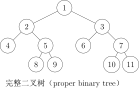
• Complete binary tree: A binary tree where only the bottom two levels may have vertices with degree less than 2, and the vertices at the bottom level are positioned as far left as possible.

  

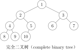
• Perfect binary tree: A binary tree where all leaves have the same depth, and every non-leaf vertex has exactly 2 children.

  

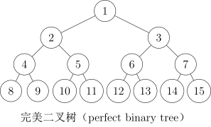
Warning

The Chinese translation of "Proper binary tree" is not fixed, and the definitions of complete binary tree and full binary tree vary across textbooks. Context must be used to determine the intended meaning.

The term "full binary tree" used by OIers often refers to a perfect binary tree.

Storage

Storing Only the Parent

Use an array parent[N] to record the parent of each vertex.

This method provides limited information and is not convenient for top-down traversal. It is often used in bottom-up dynamic programming problems.

Adjacency List

• For unrooted trees: Maintain a linear list for each vertex to record all adjacent vertices.

  std::vector<int> adj[N];
  

• For rooted trees:
  • Method 1: If the input is an undirected graph, it can still be stored as above. How to distinguish hierarchical relationships is discussed later.
  • Method 2: If the input data ensures the hierarchical relationship, this information can be utilized. Maintain a linear list for each vertex to record all its children; if needed, also record its parent in another array.

    std::vector<int> children[N];
    int parent[N];
    

    Of course, other structures (like linked lists) can replace std::vector.

Left-Child Right-Sibling Representation

Process

For rooted trees, there is a simple representation method.

First, arbitrarily order all children of each vertex.

Then, for each vertex, record two values: its first child child[u] and its next sibling sib[u]. If a vertex has no children, child[u] is empty; if it is the last child of its parent, sib[u] is empty.

Implementation

Traversing all children of a vertex can be implemented as follows.

int v = child[u];  // Start from the first child
while (v != EMPTY_NODE) {
  // ...
  // Process child v
  // ...
  v = sib[v];  // Move to the next child, i.e., a sibling of v
}

It can also be written concisely as:

for (int v = child[u]; v != EMPTY_NODE; v = sib[v]) {
  // ...
  // Process child v
  // ...
}

Binary Tree

Need to record the left and right child of each vertex.

Implementation

int parent[N];
int lch[N], rch[N];
// -- or --
int child[N][2];

Tree Traversal

DFS on Trees

DFS on a tree proceeds as follows: first visit the root, then recursively visit the subtree of each child.

This can be used to compute information such as the depth and parent of each node.

Binary Tree DFS Traversal

Preorder Traversal

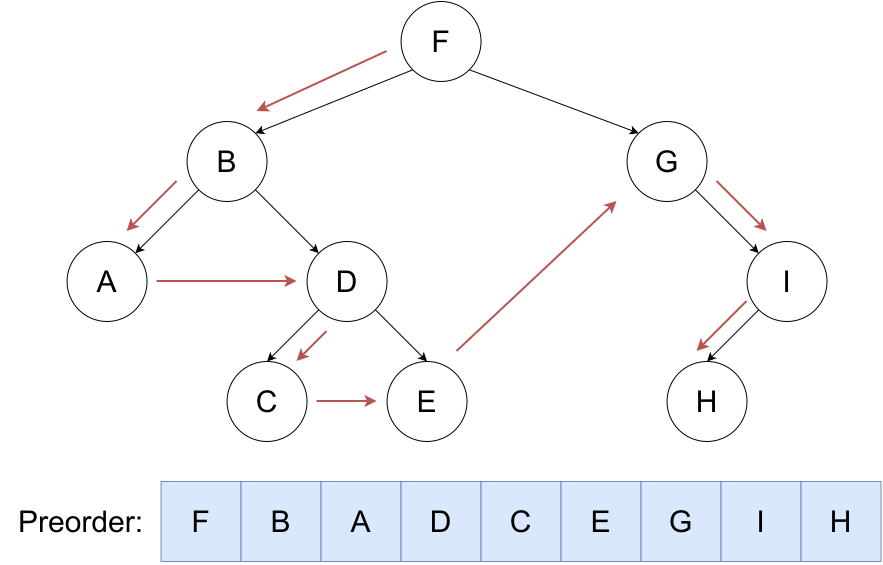
Traverse the binary tree in the order root, left, right.

Implementation

void preorder(BiTree* root) {
  if (root) {
    cout << root->key << " ";
    preorder(root->left);
    preorder(root->right);
  }
}

Inorder Traversal

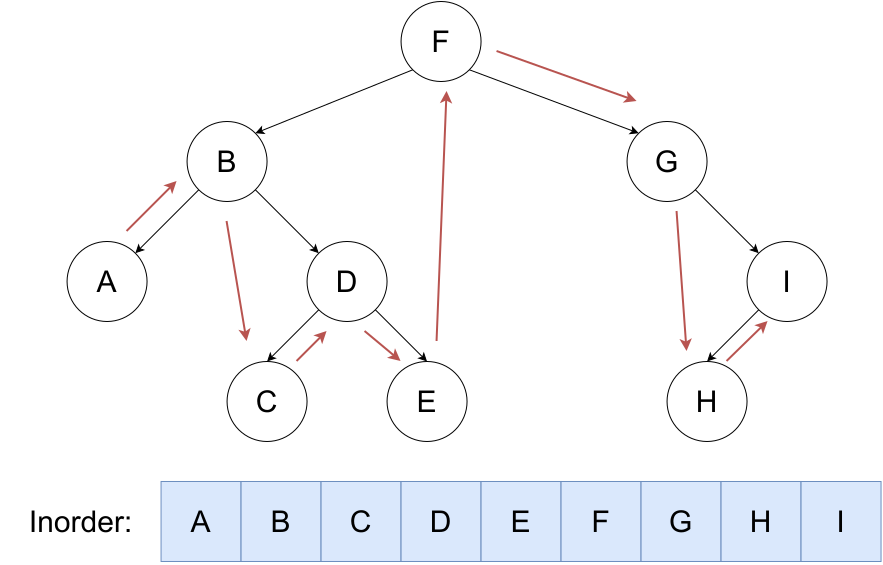
Traverse the binary tree in the order left, root, right.

Implementation

void inorder(BiTree* root) {
  if (root) {
    inorder(root->left);
    cout << root->key << " ";
    inorder(root->right);
  }
}

Postorder Traversal

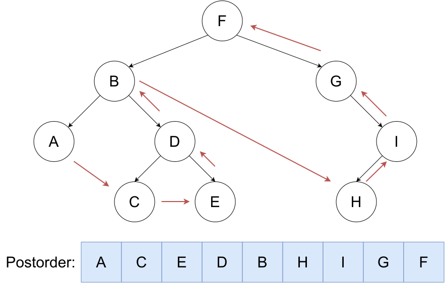
Traverse the binary tree in the order left, right, root.

Implementation

void postorder(BiTree* root) {
  if (root) {
    postorder(root->left);
    postorder(root->right);
    cout << root->key << " ";
  }
}

Reconstruction

Given the inorder traversal sequence and one other sequence (preorder or postorder), the third sequence can be reconstructed.

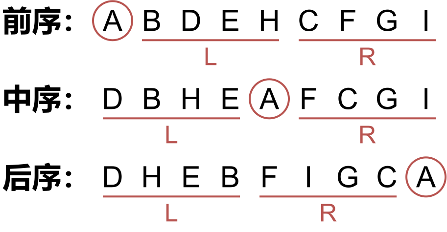
1. The first element in preorder is the root; the last element in postorder is the root.
2. First determine the root node. Then, according to the inorder sequence, nodes to the left of the root belong to the left subtree, and nodes to the right belong to the right subtree.
3. Each subtree can be treated as a new tree, following the same rules.

BFS on Trees

Start from the root and visit nodes strictly level by level.

BFS can also compute the depth and parent of each node during the process.

Level Order Traversal of a Tree

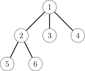
Level order traversal visits nodes layer by layer horizontally from the root to the leaves. By definition, BFS yields a level order traversal. However, level order traversal typically requires distinguishing between different levels, so the result is often represented as a two-dimensional array.

For example, the level order traversal of the tree below is [[1], [2, 3, 4], [5, 6]] (each layer from left to right).

Implementation

vector<vector<int>> levelOrder(Node* root) {
  if (!root) {
    return {};
  }
  vector<vector<int>> res;
  queue<Node*> q;
  q.push(root);
  while (!q.empty()) {
    int currentLevelSize = q.size();  // Number of nodes in the current level
    res.push_back(vector<int>());
    for (int i = 0; i < currentLevelSize; ++i) {
      Node* cur = q.front();
      q.pop();
      res.back().push_back(cur->val);
      for (Node* child : cur->children) {  // Add all children to the queue
        q.push(child);
      }
    }
  }
  return res;
}

Morris Traversal for Binary Trees

The core problem in binary tree traversal is how to return to the current node and continue traversal after visiting its children. Both recursive and non-recursive traversal methods use a stack to record the return path, enabling movement from lower levels back to upper levels. Their space complexity is \(O(\log n)\) at best and \(O(n)\) at worst (when the tree is linear).

The essence of Morris traversal is to avoid using a stack by utilizing the unused right pointers of lower-level nodes to point back to some upper-level node, thereby achieving movement from lower to upper levels.

Process of Morris Traversal

Assume we are at the current node cur, starting from the root.

1. If cur is null, stop traversal. Otherwise, proceed.
2. If cur has no left subtree, move cur to the right (cur = cur->right).
3. If cur has a left subtree, find the rightmost node in the left subtree, denoted as mostRight.
   • If the right pointer of mostRight points to null, set it to point to cur, then move cur to the left (cur = cur->left).
   • If the right pointer of mostRight points to cur, set it back to null, then move cur to the right (cur = cur->right).

For example, cur starts at node 1.

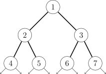
When cur visits node 2 for the first time, it finds the rightmost node 4 in the left subtree and sets the right pointer of 4 to point to cur (node 2).

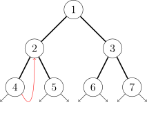
cur returns to the upper level via the right pointer of 4. When cur visits node 2 for the second time, it finds the rightmost node 4 in the left subtree, sets its right pointer back to null, and then continues to the right subtree. The subsequent process is omitted.

The overall access order of the tree is 1242513637. It can be observed that nodes with left subtrees are visited twice, while nodes without left subtrees are visited only once.

Implementation

void morris(TreeNode* root) {
  TreeNode* cur = root;
  while (cur) {
    if (!cur->left) {
      // If the current node has no left child, output its value and move to the right subtree
      std::cout << cur->val << " ";
      cur = cur->right;
      continue;
    }
    // Find the rightmost node in the left subtree of the current node
    TreeNode* mostRight = cur->left;
    while (mostRight->right && mostRight->right != cur) {
      mostRight = mostRight->right;
    }
    if (!mostRight->right) {
      // If the rightmost node's right pointer is null, set it to point to the current node and move to the left subtree
      mostRight->right = cur;
      cur = cur->left;
    } else {
      // If the rightmost node's right pointer points to the current node, the left subtree has been traversed. Output the current node's value and move to the right subtree
      mostRight->right = nullptr;
      std::cout << cur->val << " ";
      cur = cur->right;
    }
  }
}

Unrooted Trees

Process

Tree traversal is generally depth-first traversal. The most important point during this process is to avoid revisiting vertices.

Since a tree is an acyclic graph, it suffices to record which vertex the current vertex was visited from. Then, proceed to all adjacent vertices except that one to avoid repetition.

Implementation

void dfs(int u, int from) {
  // Recursively enter all children except the one from which we came (`from`)
  // For the starting vertex, `from` is empty, so all adjacent vertices are visited, as expected.
  for (int v : adj[u])
    if (v != from) {
      dfs(v, u);
    }
}

// When starting traversal
int EMPTY_NODE = -1;  // A non-existent identifier
int root = 0;         // Choose any vertex as the starting point
dfs(root, EMPTY_NODE);

Rooted Trees

For rooted trees, the hierarchical relationship between vertices needs to be distinguished.

Observing the traversal process above, if starting from the root, the value of from when visiting a vertex is the identifier of its parent.

Using this method, given an undirected input, we can compute the parent and the list of children for all vertices.

Parts of this page are adapted from the blog post Binary Tree: Preorder, Inorder, Postorder Traversal, following the CC 4.0 BY-SA license.

---

本页面最近更新：，更新历史
发现错误？想一起完善？ 在 GitHub 上编辑此页！
本页面贡献者：OI-wiki
本页面的全部内容在 CC BY-SA 4.0 和 SATA 协议之条款下提供，附加条款亦可能应用