Introduction
Link/Cut Tree is a data structure used to solve dynamic tree problems.
Link/Cut Tree, also known as Link-Cut Tree, abbreviated as LCT, is not called "dynamic tree"; dynamic tree refers to a class of problems.
Splay Tree is the foundation of LCT, but the Splay Tree used in LCT differs slightly from the ordinary Splay in details (with some extensions).
Problem Introduction
Maintain a tree supporting the following operations:
- Modify the weights on the path between two points.
- Query the sum of weights on the path between two points.
- Modify the weights of a subtree.
- Query the sum of weights of a subtree.
This is a template problem for tree chain decomposition.
But add one more operation:
- Disconnect and reconnect some edges, ensuring it remains a tree.
The answers must be computed online.
This becomes a dynamic tree problem, which can be solved using LCT.
Dynamic Tree Problems
Maintain a forest, support deleting an edge, adding an edge, and ensure the forest remains a forest after additions and deletions. We need to maintain some information about this forest.
Common operations include connectivity between two points, sum of weights on the path between two points, connecting two points, cutting an edge, modifying information, etc.
Reviewing Tree Chain Decomposition from the Perspective of LCT
- Decompose the entire tree based on subtree size and renumber the nodes.
- We find that after renumbering, continuous intervals in the form of chains are formed on the tree, and interval operations can be performed using a segment tree.
Turning to Dynamic Tree Problems
We notice that the tree decomposition we just discussed uses subtree size as the division criterion. Can we redefine a decomposition to better adapt to our dynamic tree problems?
Consider what kind of chain is needed for dynamic tree problems.
Since we are dynamically maintaining a forest, we obviously want the chain to be one we specify, so that we can use it for solving problems.
Preferred Path Decomposition
For the edges connecting a node to all its children, we choose one edge for decomposition ourselves. We call the chosen edge a preferred edge, and the other edges virtual edges. For a preferred edge, we call the child it connects to a preferred child. For a chain composed of preferred edges, we similarly call it a preferred chain. Remember the most important reason we choose preferred path decomposition: it is chosen by us, flexible and variable. It is precisely this flexibility and variability that leads us to use Splay Trees to maintain these preferred chains.
LCT
We can simply understand LCT as using some Splay Trees to maintain dynamic tree chain decomposition, aiming to achieve interval operations on dynamic trees. For each preferred chain, we build a Splay Tree to maintain the information of the entire chain interval.
Auxiliary Tree
Let's first look at some properties of the auxiliary tree, and then understand its specific structure through a diagram.
In this article, you can think of some Splay Trees forming an auxiliary tree, each auxiliary tree maintains a tree, and some auxiliary trees constitute the LCT, which maintains the entire forest.
- The auxiliary tree consists of multiple Splay Trees, each Splay Tree maintains a path in the original tree, and the in-order traversal sequence of this Splay Tree corresponds, from front to back, to a path in the original tree "from top to bottom".
- Each node in the original tree corresponds one-to-one with a Splay node in the auxiliary tree.
- The Splay Trees in the auxiliary tree are not independent. The parent node of the root of each Splay Tree should be empty, but in LCT, the parent node of the root of each Splay Tree points to the parent node of this chain in the original tree (i.e., the parent node of the topmost point of the chain). This type of parent link differs from the usual Splay parent link in that the child recognizes the parent, but the parent does not recognize the child, corresponding to a virtual edge in the original tree. Therefore, each connected component has exactly one node whose parent is empty.
- Due to the above properties of the auxiliary tree, we do not need to maintain the original tree for any operation; the auxiliary tree can uniquely represent an original tree under any circumstances. We only need to maintain the auxiliary tree.
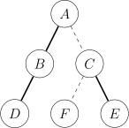
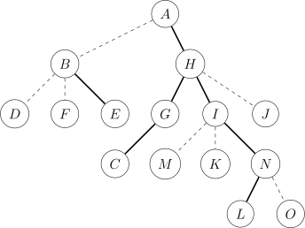
Now we have an original tree, as shown in the figure. (Bold edges are preferred edges, dashed edges are virtual edges.)
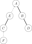
According to the definition just given, the structure of the auxiliary tree is as shown in the figure.
Considering the Structural Relationship Between the Original Tree and the Auxiliary Tree
- Preferred chains in the original tree: In the auxiliary tree, all nodes are in one Splay Tree.
- Virtual chains in the original tree: In the auxiliary tree, the Father of the Splay containing the child node points to the parent node, but neither of the parent node's children point to the child node.
- Note: The root of the original tree is not equal to the root of the auxiliary tree.
- The Father pointer in the original tree is not equal to the Father pointer in the auxiliary tree.
- The auxiliary tree can arbitrarily change roots while satisfying the properties of the auxiliary tree and Splay Trees.
- Transformations between preferred and virtual chains can be easily performed on the auxiliary tree, which implements dynamic maintenance of tree chain decomposition.
Variable Declarations to Be Used Next
ch[N][2]left and right childrenf[N]parent pointersum[N]path weight sumval[N]node weighttag[N]flip marklaz[N]weight marksiz[N]subtree size in the auxiliary tree- Other_Vars
Function Declarations
General Data Structure Functions (literal meaning)
PushUp(x)PushDown(x)
Splay Tree Functions
Below are the functions used in the Splay Tree; for details, refer to Splay Tree.
Get(x)gets which child \(x\) is of its parent.Splay(x)through interaction with the Rotate operation, rotates \(x\) to the root of the current Splay.Rotate(x)rotates \(x\) up one level.
New Operations
Access(x)places all points from the root to \(x\) on a preferred chain, making the path from the root to \(x\) a preferred path, and within the same Splay Tree. Only this operation is mandatory; other operations are implemented depending on the problem.IsRoot(x)determines whether \(x\) is the root of its tree.Update(x)after theAccessoperation, recursivelyPushDownupdates information from top to bottom.MakeRoot(x)makes node \(x\) the root of its tree.Link(x, y)connects an edge between points \(x\) and \(y\).Cut(x, y)deletes the edge between points \(x\) and \(y\).Find(x)finds the root node ID of the tree containing \(x\).Fix(x, v)modifies the weight of node \(x\) to \(v\).Split(x, y)extracts the path between \(x\) and \(y\), facilitating interval operations.
Macro Definitions
#define ls ch[p][0]#define rs ch[p][1]
Function Explanations
PushUp()
1 2 3 4 | |
PushDown()
1 2 3 4 5 6 | |
Splay() && Rotate()
Here Splay() and Rotate() differ somewhat from the implementation in a Splay Tree.
1 2 3 4 5 6 7 8 9 10 11 12 13 14 15 16 17 18 | |
The above functions can be found in Splay Tree.
Below are functions unique to LCT.
isRoot()
1 2 3 | |
Access()
1 2 3 4 5 6 7 8 9 10 | |
-
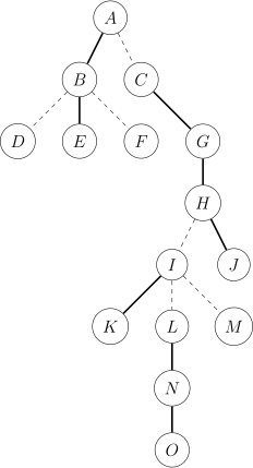
We have a tree like this, solid lines are preferred edges, dashed lines are virtual edges.
-
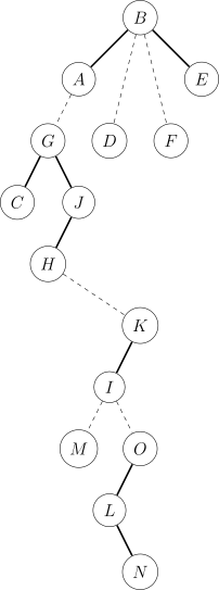
Its auxiliary tree might look like this (different construction methods may lead to different LCT structures).
-
Now we want to
Access(N), turning all edges on the path from \(A\) to \(N\) into preferred edges, pulling them into one Splay Tree.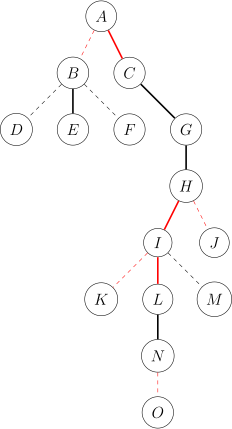
-
The implementation method is to update the Splay step by step from bottom to top.
-
First, we rotate \(N\) to the root of the current Splay.
-
To maintain the properties of the AuxTree (auxiliary tree), the original preferred edge \(N\)—\(O\) must be changed to a virtual edge.
-
Due to the property of recognizing parent but not child, we can unilaterally set \(N\)'s child to
NULL. -
Thus, the original AuxTree changes from the figure below to the one after.
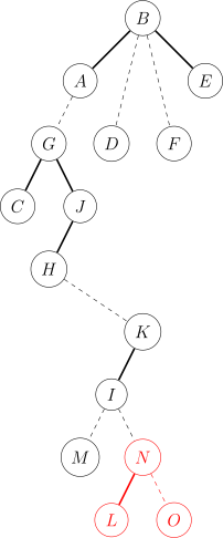
-
Next, we rotate the Father \(I\) pointed to by \(N\) to the root of \(I\)'s Splay Tree.
-
The original preferred edge \(I\)—\(K\) needs to be removed. At this point, we set \(I\)'s right child to \(N\), obtaining an Splay like \(I\)—\(L\).
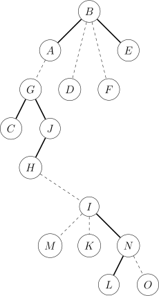
-
Next, following the same steps, since \(I\)'s Father points to \(H\), we rotate \(H\) to the root of its Splay Tree, then set \(H\)'s rs to \(I\).
-
The resulting tree is as follows.
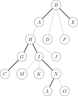
-
Similarly, we
Splay(A)and set \(A\)'s right child to \(H\). -
Thus we obtain such an AuxTree. And we find that the entire path \(A\)—\(N\) is already in the same Splay Tree.
1 2 3 4 5 6 7 8 | |
We find that Access() is actually quite simple, with only the following four steps:
- Rotate the current node to the root.
- Replace the child with the previous node.
- Update the current node's information.
- Replace the current node with its parent and continue.
The Access provided here also has a return value. This return value is equivalent to the ID of the parent node of the virtual edge during the last preferred-virtual chain transformation. This value has two meanings:
- When performing two consecutive
Accessoperations, the return value of the secondAccessoperation equals the LCA of these two nodes. - Represents the root of the Splay Tree containing the chain from \(x\) to the root. This node must have been rotated to the root, and its parent must be empty.
Update()
1 2 3 4 5 | |
makeRoot()
- The importance of
Make_Root()is no less than that ofAccess(). When we need to maintain path information, situations will inevitably arise where path depth is not strictly increasing. According to the properties of AuxTree, such paths cannot appear in a Splay Tree. - At this point, we need to use
Make_Root(). - The role of
Make_Root()is to make the specified point the root of the original tree. Consider how to implement this operation. - Let the return value of
Access(x)be \(y\). Then the path from \(x\) to the current root exactly forms a Splay, and the root of this Splay is \(y\). - Consider representing the tree as a directed graph, assigning a direction to each edge, indicating the direction from child to parent. It's easy to see that changing the root is equivalent to reversing all edges on the path from \(x\) to the root (think carefully).
- Therefore, simply flip the path from \(x\) to the current root.
- Since \(y\) is the root of the Splay representing the path from \(x\) to the current root, we can perform an interval flip on the Splay Tree rooted at \(y\).
1 2 3 4 5 | |
Link()
- Linking two points is actually very simple. First
Make_Root(x), then set \(x\)'s parent to point to \(y\). Obviously, this operation cannot occur within the same tree, so remember to check first.
1 2 3 4 5 | |
Split()
- The
Splitoperation is straightforward: it extracts a Splay Tree maintaining the path from \(x\) to \(y\). - First
MakeRoot(x), thenAccess(y). If you want \(y\) as the root, thenSplay(y). - Additionally, these three operations of Split can directly bring the required path into \(y\)'s subtree, allowing other operations.
Cut()
Cuthas two scenarios: guaranteed to be legal and not necessarily guaranteed to be legal.- If legality is guaranteed, simply
Split(x, y). At this point, \(y\) is the root, and \(x\) must be its child; disconnect both directions. Like this:
1 | |
If legality is not guaranteed, we need to check if the edge exists. Here we can use a map to store edges, but there is also a method using properties:
To delete an edge, the following three conditions must be met:
- \(x,y\) are connected.
- There are no other chains on the path between \(x\) and \(y\).
- \(x\) has no right child.
In summary, the meaning of the above three sentences is one: there is an edge between \(x\) and \(y\).
The specific implementation is left as an exercise. Checking connectivity requires using Find mentioned later; for the other two points, think a bit about the structure to know how to judge.
Find()
Find()finds the root of the original tree containing \(x\). Do not confuse the original tree root with the auxiliary tree root. AfterAccess(p), thenSplay(p). The root is then the one with the smallest depth in the tree; keep going to the left child,PushDownalong the way.- Keep going until there is no ls, very simple.
- Note: after each query, you need to
Splaythe node corresponding to the answer to ensure complexity.
1 2 3 4 5 6 7 8 | |
Notes
- Before any operation, always think about whether
PushUporPushDownis needed. Due to the special flexibility of LCT, missing onePushdownorPushupmight modify points that shouldn't be modified! - LCT's
Rotateis somewhat different from Splay's;if (z)must be placed first. - LCT's
Splayoperation rotates to the root; there is no operation to rotate to someone's child, because it's not needed.
Time Complexity
Most operations in LCT are based on Access, and the time complexity of other operations is constant. Therefore, we only need to analyze the time complexity of the Access operation.
The time complexity of Access mainly comes from multiple splay operations and accessing virtual edges on the path. We analyze the time complexity of these two parts separately.
-
splay
-
Define \(w(x) = \log size(x)\), where \(size(x)\) represents the sum of all virtual and preferred edges rooted at \(x\).
-
Define potential function \(\Phi = \sum_{x \in T} w(x)\), where \(T\) represents the set of all nodes.
From the time complexity analysis of Splay, it is known that the amortized time complexity of the splay operation is \(O(\log n)\).
-
-
Accessing virtual edges
Referring to Heavy-Light Decomposition, define two types of virtual edges:
-
Heavy virtual edge: A virtual edge from node \(v\) to its parent, where \(size(v) > \frac{1}{2} size(parent(v))\).
-
Light virtual edge: A virtual edge from node \(v\) to its parent, where \(size(v) \leq \frac{1}{2} size(parent(v))\).
For handling virtual edges, potential analysis can be used. Define the potential function \(\Phi\) as the number of all heavy virtual edges. Define the amortized cost \(c_i = t_i + \Delta \Phi_i\), where \(t_i\) is the actual operation cost, and \(\Delta \Phi_i\) is the change in potential.
-
After traversing a heavy virtual edge, it is converted into a preferred edge. This operation reduces the potential by \(1\), as it optimizes the tree structure by strengthening important connections. Since its actual operation cost is \(O(1)\), it offsets the increase in potential, so it does not increase the amortized cost. All amortized cost is concentrated on handling light virtual edges.
-
Each
Accessoperation traverses at most \(O(\log n)\) light virtual edges, thus consuming at most \(O(\log n)\) actual operation cost, converting to \(O(\log n)\) heavy virtual edges, i.e., the potential increases at a cost of \(O(\log n)\).
Thus, the final amortized complexity of accessing virtual edges is the sum of the actual operation cost and the potential change, i.e., \(O(\log n)\).
-
In summary, the time complexity of the Access operation in LCT is the sum of the splay and virtual edge access complexities. Therefore, the final amortized complexity is \(O(\log n)\). That is, for an LCT with n nodes, performing m Access operations has a time complexity of \(O(n \log n + m \log n)\). Consequently, operations based on Access such as Cut, Link, Findroot also have an amortized complexity of \(O(\log n)\).
Exercises
Maintaining Tree Path Information
LCT can extract the path from point \(x\) to point \(y\) on the tree into a Splay rooted at \(y\) through the Split(x,y) operation. Modifying and querying tree path information becomes operations on a balanced tree, giving LCT an advantage in maintaining tree path information. Additionally, binary search on tree paths implemented with LCT has one less \(O(\log n)\) factor compared to tree chain decomposition.
Example 「National Training Team」Tree II
Given a tree with \(n\) nodes, each node's initial weight is \(1\). Perform \(q\) operations, each being one of the following four types:
- u1 v1 u2 v2: Delete the edge between \(u_1,v_1\) on the tree, connect \(u_2,v_2\), ensuring the operation is legal and the graph remains a tree after connection.+ u v c: Increase the weights of all nodes on the path between \(u,v\) on the tree by \(c\).* u v c: Multiply the weights of all nodes on the path between \(u,v\) on the tree by \(c\).-
/ u v: Output the sum of weights of nodes on the path between \(u,v\) on the tree modulo \(51061\).\(1\le n,q\le 10^5,0\le c\le 10^4\)
The
-operation can be directlyCut(u1,v1),Link(u2,v2).
When modifying the path between \(u,v\) on the tree, first Split(u,v).
This problem requires performing subtree addition, subtree multiplication, and subtree summation on the auxiliary tree. So besides the subtree flip mark that general LCT needs to maintain, we also need to maintain subtree addition and multiplication marks. The method of handling marks is the same as in Splay.
When applying and pushing down addition marks, the change in subtree weight sum is related to the number of nodes in the subtree, so we also need to maintain subtree size siz.
When pushing down marks, order matters: push down multiplication marks first, then addition marks. Subtree flip and subtree addition/multiplication marks do not conflict.
Reference Code
1 2 3 4 5 6 7 8 9 10 11 12 13 14 15 16 17 18 19 20 21 22 23 24 25 26 27 28 29 30 31 32 33 34 35 36 37 38 39 40 41 42 43 44 45 46 47 48 49 50 51 52 53 54 55 56 57 58 59 60 61 62 63 64 65 66 67 68 69 70 71 72 73 74 75 76 77 78 79 80 81 82 83 84 85 86 87 88 89 90 91 92 93 94 95 96 97 98 99 100 101 102 103 104 105 106 107 108 109 110 111 112 113 114 115 116 117 118 119 120 121 122 123 124 125 126 127 128 129 130 131 132 133 134 135 136 137 138 139 140 141 142 143 144 145 146 147 148 149 150 151 152 153 154 | |
Exercises
Maintaining Connectivity Properties
Checking Connectivity
Using LCT's Find() function, we can check whether two points in a dynamic forest are connected. If Find(x)==Find(y), then points \(x,y\) are in the same tree and connected.
Example 「SDOI2008」Cave Survey
Initially there are \(n\) independent points, \(m\) operations. Each operation is one of the following:
Connect u v: Connect an edge between points \(u,v\).Destroy u v: Delete the edge between \(u,v\), guaranteed such an edge existed before.Query u v: Ask whether \(u,v\) are connected.
Guarantee that the graph is always a forest at any time.
\(n\le 10^4, m\le 2\times 10^5\)
Reference Code
1 2 3 4 5 6 7 8 9 10 11 12 13 14 15 16 17 18 19 20 21 22 23 24 25 26 27 28 29 30 31 32 33 34 35 36 37 38 39 40 41 42 43 44 45 46 47 48 49 50 51 52 53 54 55 56 57 58 59 60 61 62 63 64 65 66 67 68 69 70 71 72 73 74 75 76 77 78 79 80 81 82 83 84 85 86 87 88 | |
Maintaining Edge Biconnected Components
If edge biconnected components need to be contracted into points, each time an edge is added, if the two points connected on the tree are already connected, then all points on this path will be merged into one point.
Example 「AHOI2005」Route Planning
Given \(n\) points, initially with \(m\) undirected edges, \(q\) operations, each being one of the following:
0 u v: Delete the edge between \(u,v\), guaranteed such an edge exists at this time.1 u v: Query the number of edges that must be passed through by all possible paths between \(u,v\) at this time.
Guarantee the graph is connected at any time.
\(1<n<3\times 10^4,1<m<10^5,0\le q\le 4\times 10^4\)
It can be found that the number of edges that must be passed through by all possible paths between \(u,v\) equals the number of nodes on the path between the contracted point containing \(u\) and the contracted point containing \(v\) after contracting all edge biconnected components into points, minus \(1\).
Since the delete edge operation in the problem is difficult to handle, we consider offline reverse operations, changing delete edge to add edge.
When adding an edge, if the two points were not originally connected, connect them in LCT; otherwise, extract the path between these two points in LCT before adding this edge, traverse the subtree on the auxiliary tree, which is equivalent to traversing this path, merge these points, and use a union-find set to maintain the merged information.
Replace the path on the tree with the representative element of the merged union-find set. Note that every subsequent operation must find the representative element of the operation point in the union-find set to perform the operation.
Reference Code
1 2 3 4 5 6 7 8 9 10 11 12 13 14 15 16 17 18 19 20 21 22 23 24 25 26 27 28 29 30 31 32 33 34 35 36 37 38 39 40 41 42 43 44 45 46 47 48 49 50 51 52 53 54 55 56 57 58 59 60 61 62 63 64 65 66 67 68 69 70 71 72 73 74 75 76 77 78 79 80 81 82 83 84 85 86 87 88 89 90 91 92 93 94 95 96 97 98 99 100 101 102 103 104 105 106 107 108 109 110 111 112 113 114 115 116 117 118 119 120 121 122 123 124 125 126 127 128 129 130 131 132 133 134 135 136 137 138 139 140 141 142 143 144 145 146 147 148 149 150 151 152 153 154 155 156 157 158 159 160 161 162 163 164 165 166 167 168 169 | |
Exercises
Maintaining Edge Weights
LCT cannot directly handle edge weights. At this point, a corresponding point needs to be created for each edge to facilitate querying edge information on chains. Using this technique, spanning trees can be dynamically maintained.
Example luogu P4234 Minimum Difference Spanning Tree
Given a weighted undirected graph with \(n\) points and \(m\) edges, find the spanning tree where the difference between the maximum edge weight and the minimum edge weight is minimized, and output this difference.
Guarantee at least one spanning tree exists.
\(1\le n\le 5\times 10^4,1\le m\le 2\times 10^5,1\le w_i\le 10^4\)
Sort edges in ascending order of edge weight, enumerate the rightmost edge selected. To obtain the optimal solution, the edge weight of the minimum edge needs to be maximized.
Add edges in order each time. If the two points to be connected are already connected, delete the edge with the smallest weight between these two points. If the entire graph has become a connected tree, update the answer with the current edge weight minus the minimum edge weight. The minimum edge weight can be updated using the two-pointer method.
LCT does not have fixed parent-child relationships, so edge weights cannot be recorded in node weights.
To record edge information on tree chains, edge splitting can be used. Create a corresponding point for each edge, connect an edge from this point to its two endpoints. The original connect and delete edge operations become two operations each.
Reference Code
1 2 3 4 5 6 7 8 9 10 11 12 13 14 15 16 17 18 19 20 21 22 23 24 25 26 27 28 29 30 31 32 33 34 35 36 37 38 39 40 41 42 43 44 45 46 47 48 49 50 51 52 53 54 55 56 57 58 59 60 61 62 63 64 65 66 67 68 69 70 71 72 73 74 75 76 77 78 79 80 81 82 83 84 85 86 87 88 89 90 91 92 93 94 95 96 97 98 99 100 101 102 103 104 105 106 107 108 109 110 111 112 113 114 115 116 117 118 119 120 121 122 123 124 125 126 127 128 129 130 131 132 133 134 135 136 137 138 139 140 141 142 143 144 145 146 | |
Exercises
Maintaining Subtree Information
LCT is not good at maintaining subtree information. By aggregating information from all virtual subtrees of a node, the information of the entire tree can be obtained.
Example 「BJOI2014」Great Fusion
Given \(n\) nodes and \(q\) operations, each operation is of the following form:
A x yConnect an edge between nodes \(x\) and \(y\).Q x yGiven an existing edge \((x,y)\), find how many simple paths contain edge \((x,y)\).
Guarantee that at any time, the graph is a forest.
\(1\le n,q,x,y\le 10^5\)
Consider another formulation for query Q. We find the answer equals the product of the number of nodes on the \(x\) side of edge \((x,y)\) and the number of nodes on the \(y\) side, i.e., the number of nodes in the trees containing \(x\) and \(y\) respectively after disconnecting edge \((x,y)\). To eliminate the effect of edge deletion, we reconnect edge \((x,y)\) after the query.
The operations in the problem include both connecting and deleting edges, and guarantee a forest at any time, which naturally leads us to think of using LCT for maintenance. However, in this problem, LCT maintains subtree sizes, unlike the usual maintenance of chain information. Moreover, LCT's structure recognizes parent but not child, making direct subtree statistics inconvenient. What to do?
The method is to aggregate the contributions of all virtual children (i.e., children whose parent is \(x\), but \(x\)'s left and right children in the Splay do not include them) of a node \(x\).
Define \(siz2[x]\) as the total number of nodes in all virtual subtrees of node \(x\), and \(siz[x]\) as the number of nodes in the subtree of node \(x\).
Different from the usual method of maintaining subtree node counts in Splay, when calculating the number of nodes in the subtree of node \(x\), we also add \(siz2[x]\), i.e.,
1 2 3 4 | |
Moreover, when we change the shape of the Splay (i.e., change a node's left and right child pointers in the Splay), we need to update the value of \(siz2[x]\) in a timely manner.
In the Rotate(),Splay() operations, we only change the relative positions of nodes in the Splay, without changing the virtual/real status of any edge, so no modification to \(siz2[x]\) is made.
In the access operation, after each splay, the right child of the just splayed node changes, meaning the virtual/real status of the edge between this node and its original right child, and the edge between this node and its new right child, changes. We need to add the contribution of the subtree that just became virtual, and subtract the contribution of the subtree that just became real. The code is as follows:
1 2 3 4 | |
In the MakeRoot(),Find() operations, we only call previous functions or traverse edges on the Splay, no modifications are needed.
When connecting two points, we modify the parent of a node. We need to add the subtree size contribution of the new child to the \(siz2\) value of the parent node.
1 2 3 4 | |
When disconnecting an edge, we only delete a real edge on the Splay; the Maintain operation will maintain this information, no modification is needed.
The above are details of code modifications. Finally, summarize the requirements and methods for LCT to maintain subtree information:
- The maintained information must have subtractivity, such as subtree node count, subtree weight sum, but cannot directly maintain subtree maximum/minimum, because when converting a virtual edge to a real edge, the contribution of the original virtual edge must be excluded.
- Create an additional value to store the contribution of virtual subtrees. Include it in the node's answer when aggregating, and maintain it timely when the virtual/real status of edges changes.
- The rest is the same as ordinary LCT. When aggregating subtree information, always treat it as the root node.
- If the maintained information does not have subtractivity, such as maintaining interval maximum/minimum, you can open a balanced tree for each node to maintain the maximum/minimum in the node's virtual subtrees.
Reference Code
```cpp
include
include
include
using namespace std; constexpr int MAXN = 100010; using ll = long long;
struct Splay { int ch[MAXN][2], fa[MAXN], siz[MAXN], siz2[MAXN], tag[MAXN];
void clear(int x) { ch[x][0] = ch[x][1] = fa[x] = siz[x] = siz2[x] = tag[x] = 0; }
int getch(int x) { return ch[fa[x]][1] == x; }
int isroot(int x) { return ch[fa[x]][0] != x && ch[fa[x]][1] != x; }
void maintain(int x) {
  clear(0);
  if (x) siz[x] = siz[ch[x][0]] + 1 + siz[ch[x][1]] + siz2[x];
}
void pushdown(int x) { if (tag[x]) { if (ch[x][0]) swap(ch[ch[x][0]][0], ch[ch[x][0]][1]), tag[ch[x][0]] ^= 1; if (ch[x][1]) swap(ch[ch[x][1]][0], ch[ch[x][1]][1]), tag[ch[x][1]] ^= 1; tag[x] = 0; } }
void update(int x) { if (!isroot(x)) update(fa[x]); pushdown(x); }
void rotate(int x) { int y = fa[x], z = fa[y], chx = getch(x), chy = getch(y); fa[x] = z; if (!isroot(y)) ch[z][
本页面最近更新:,更新历史
发现错误?想一起完善? 在 GitHub 上编辑此页!
本页面贡献者:OI-wiki
本页面的全部内容在 CC BY-SA 4.0 和 SATA 协议之条款下提供,附加条款亦可能应用