Quadratic Residue

Introduction

Quadratic residues can be considered as discussing the feasibility of square root operations modulo a prime. For higher-degree roots, refer to k-th residues.

Definition

Quadratic Residue

Let integers \(a\), \(p\) satisfy \((a,p)=1\). If there exists an integer \(x\) such that

\[ x^2\equiv a\pmod p, \]

then \(a\) is called a quadratic residue modulo \(p\); otherwise, \(a\) is called a quadratic non-residue modulo \(p\). In the following, when the modulus \(p\) is clear from context, we may simply write quadratic (non-)residue.

Euler's Criterion

When the modulus is an odd prime, we have the following theorem:

Euler's Criterion

For an odd prime \(p\) and an integer \(a\) satisfying \((a,p)=1\), we have

\[ a^{\frac{p-1}{2}}\equiv\begin{cases} 1 \pmod p, & (\exists x\in\mathbf{Z}),~~a\equiv x^2\pmod p,\\ -1 \pmod p, & \text{otherwise}.\\ \end{cases} \]

That is, for such \(p\) and \(a\),

1. \(a\) is a quadratic residue modulo \(p\) if and only if \(a^{\frac{p-1}{2}}\equiv 1 \pmod p\).
2. \(a\) is a quadratic non-residue modulo \(p\) if and only if \(a^{\frac{p-1}{2}}\equiv -1 \pmod p\).

Proof

First, by Fermat's Little Theorem, we have \(a^{p-1}\equiv 1\pmod p\), so

\[ \left(a^{\frac{p-1}{2}}+1\right)\left(a^{\frac{p-1}{2}}-1\right)\equiv 0\pmod p, \]

thus for any \(a\) satisfying \((a,p)=1\), we have \(a^{(p-1)/2}\equiv \pm 1\pmod p.\)

Moreover, since \(p\) is an odd prime, we have:

\[ x^{p-1}-a^{\frac{p-1}{2}}={\left(x^2\right)}^{\frac{p-1}{2}}-a^{\frac{p-1}{2}}=(x^2-a)P(x), \]

where \(P(x)\) is some integer-coefficient polynomial, and thus:

\[ \begin{aligned} x^p-x&=x\left(x^{p-1}-a^{\frac{p-1}{2}}\right)+x\left(a^{\frac{p-1}{2}}-1\right)\\ &=(x^2-a)xP(x)+\left(a^{\frac{p-1}{2}}-1\right)x.\\ \end{aligned} \]

By Theorem 5 of congruence equations, \(a\) is a quadratic residue modulo \(p\) if and only if \(a^{(p-1)/2}\equiv 1\pmod p\). Consequently, \(a\) is a quadratic non-residue modulo \(p\) if and only if \(a^{(p-1)/2}\equiv -1\pmod p\).

Based on Euler's criterion, we can derive the following corollary:

Number of Quadratic Residues

For an odd prime \(p\), there are exactly \(\dfrac{p-1}{2}\) quadratic residues and \(\dfrac{p-1}{2}\) quadratic non-residues modulo \(p\).

Proof

According to Euler's criterion, consider \(a^{\frac{p-1}{2}}\equiv 1\pmod p.\)

Note that \(\dfrac{p-1}{2}\mid (p-1)\). By Theorem 6 of congruence equations, \(a^{\frac{p-1}{2}}\equiv 1\pmod p\) has \(\dfrac{p-1}{2}\) solutions. Therefore, modulo \(p\), there are \(\dfrac{p-1}{2}\) quadratic residues and \(\dfrac{p-1}{2}\) quadratic non-residues.

Legendre Symbol

For convenience in further discussion, we introduce the following notation:

Legendre Symbol

For an odd prime \(p\) and an integer \(a\), define the Legendre symbol as:

\[ \left(\frac{a}{p}\right)=\begin{cases} 0, & p\mid a,\\ 1, & (p\nmid a) \land ((\exists x\in\mathbf{Z}),~~a\equiv x^2\pmod p),\\ -1, & \text{otherwise}.\\ \end{cases} \]

That is, for \(a\) with \((a,p)=1\),

• \(a\) is a quadratic residue modulo \(p\) if and only if \(\left(\dfrac{a}{p}\right)=1.\)
• \(a\) is a quadratic non-residue modulo \(p\) if and only if \(\left(\dfrac{a}{p}\right)=-1.\)

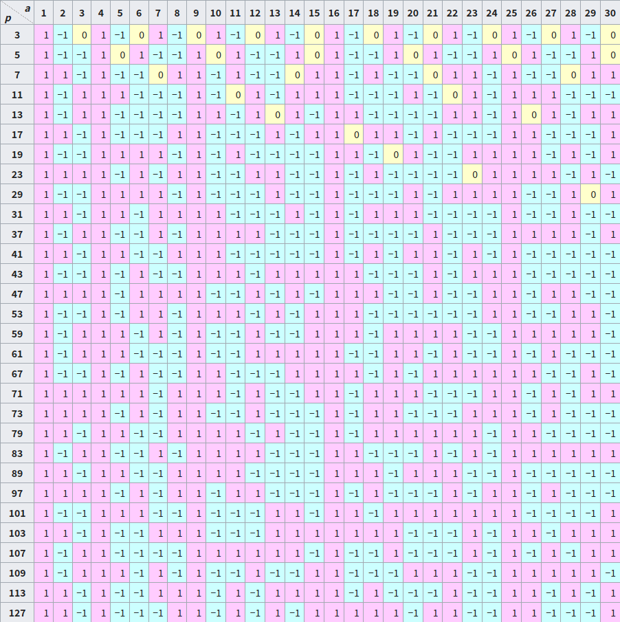
The following table shows values of the Legendre symbol for some small primes (From Wikipedia):

Properties

1. For any integer \(a\),

   \[ a^{\frac{p-1}{2}}\equiv \left(\frac{a}{p}\right)\pmod p. \]

   Further, we have the corollaries:

   • \[ \left(\dfrac{1}{p}\right)=1. \]
   • \[ \left(\dfrac{-1}{p}\right)=(-1)^{\frac{p-1}{2}}=\begin{cases} 1, & p\equiv 1\pmod 4,\\ -1, & p\equiv 3\pmod 4. \end{cases} \]

2. \(a_1\equiv a_2\pmod p\implies \left(\dfrac{a_1}{p}\right)=\left(\dfrac{a_2}{p}\right).\)

3. (Complete multiplicativity) For any integers \(a_1,a_2\),

   \[ \left(\frac{a_1a_2}{p}\right)=\left(\frac{a_1}{p}\right)\left(\frac{a_2}{p}\right). \]

   We have the corollary: for integers \(a,b\) with \(p\nmid b\),

   \[ \left(\frac{ab^2}{p}\right)=\left(\frac{a}{p}\right). \]
4. \[ \left(\frac{2}{p}\right)=(-1)^{\frac{p^2-1}{8}}=\begin{cases} 1, & p\equiv \pm 1\pmod 8, \\ -1, & p\equiv \pm 3\pmod 8. \\ \end{cases} \]

Proof

1. Follows directly from the definition of the Legendre symbol and Euler's criterion.

2. Note that

   \[ a_1\equiv a_2\pmod p\implies \left(\frac{a_1}{p}\right)\equiv\left(\frac{a_2}{p}\right)\pmod p, \]

   and \(\left|\left(\dfrac{a_1}{p}\right)-\left(\dfrac{a_2}{p}\right)\right|\leq 2\) with \(p>2\), so:

   \[ a_1\equiv a_2\pmod p\implies \left(\frac{a_1}{p}\right)=\left(\frac{a_2}{p}\right). \]

3. From 1,

   \[ \left(\frac{a_1a_2}{p}\right)\equiv a_1^{\frac{p-1}{2}}a_2^{\frac{p-1}{2}}\equiv\left(\frac{a_1}{p}\right)\left(\frac{a_2}{p}\right)\pmod p. \]

   Since \(\left|\left(\dfrac{a_1a_2}{p}\right)-\left(\dfrac{a_1}{p}\right)\left(\dfrac{a_2}{p}\right)\right|\leq 2\) and \(p>2\), we have

   \[ \left(\frac{a_1a_2}{p}\right)=\left(\frac{a_1}{p}\right)\left(\frac{a_2}{p}\right). \]

4. See Quadratic Reciprocity

Based on these properties, if we can compute \(\left(\dfrac{p}{q}\right)\) for any odd primes \(p\) and \(q\), then we can compute the Legendre symbol for any valid case. Next, we have an elegant theorem that cleverly establishes a connection between \(\left(\dfrac{p}{q}\right)\) and \(\left(\dfrac{q}{p}\right)\), allowing us to compute it using a method similar to the Euclidean algorithm.

Quadratic Reciprocity

Quadratic Reciprocity Law

Let \(p\), \(q\) be two distinct odd primes. Then

\[ \left(\frac{p}{q}\right)\left(\frac{q}{p}\right)=(-1)^{\frac{p-1}{2}\frac{q-1}{2}}. \]

There are many proofs¹. One proof is based on the following lemma²:

Gauss's Lemma

Let \(p\) be an odd prime, \((n,p)=1\). For integers \(k~\left(1\leq k\leq (p-1)/2\right)\), let \(r_k=nk\bmod p\). Define \(A=\{r_k:r_k < p/2\}\), \(B=\{r_k:r_k > p/2\}\). Then

\[ \left(\frac{n}{p}\right)=(-1)^{|B|}. \]

Proof

Let \(\lambda=|A|\), \(\mu=|B|\). Clearly \(\lambda+\mu=(p-1)/2\). Then

\[ n^{\frac{p-1}{2}}\left(\frac{p-1}{2}\right)!=\prod_{k=1}^{\frac{p-1}{2}} nk\equiv\prod_{a\in A}a\prod_{b\in B}b\pmod{p}. \]

For any \(b\in B\), we have \(\dfrac{p}{2} < b < p\), so \(0 < p-b < \dfrac{p}{2}\). Moreover, for any \(b\in B\), we have \(p-b\notin A\); otherwise, if there exist \(a\in A\) and \(b\in B\) such that \(a=p-b\), then there exist integers \(0 < k_1,k_2 < (p-1)/2\) such that \(a=nk_1\), \(b=nk_2\) and \(p\mid n(k_1+k_2)\). Since \((n,p)=1\), we have \(p\mid (k_1+k_2)\). Noting that \(0 < k_1+k_2 < p\), we get a contradiction. Therefore,

\[ n^{\frac{p-1}{2}}\left(\frac{p-1}{2}\right)!\equiv(-1)^{\mu}\prod_{a\in A}a\prod_{b\in B}(p-b)=(-1)^{\mu}\left(\frac{p-1}{2}\right)!\pmod{p}, \]

i.e.,

\[ n^{\frac{p-1}{2}}\equiv(-1)^{\mu}\pmod{p}. \]

The result then follows from Property 1 of the Legendre symbol.

Generalization

Gauss's Lemma can be generalized as follows⁷:

Let \(p\) be an odd prime, and let \(I\subset\mathbf{Z}_p^*\) satisfy \(I\cup -I=\mathbf{Z}_p^*\) and \(I\cap -I=\varnothing\), where \(-I:=\{-i:i\in I\}\). Then for any integer \(n\) coprime to \(p\),

\[ \left(\frac{n}{p}\right)=(-1)^{|J|}, \]

where \(J=\{j\in I:nj\in -I\}\).

It is easy to see that taking \(I=\{1,2,\dots,(p-1)/2\}\) yields Gauss's Lemma. The proof is essentially the same as that of Gauss's Lemma, so it is omitted.

We can easily obtain the following corollary:

Corollary

For an odd prime \(p\),

\[ \left(\frac{2}{p}\right)=(-1)^{\frac{p^2-1}{8}}=\begin{cases} 1, & p\equiv \pm 1\pmod 8, \\ -1, & p\equiv \pm 3\pmod 8. \\ \end{cases} \]

For an odd prime \(p\) and an odd integer \(n\) with \((n,p)=1\),

\[ \left(\frac{n}{p}\right)=(-1)^{\sum_{i=1}^{(p-1)/2}\lfloor ni/p \rfloor}. \]

Proof

For \(n,k,r_k,A,B,\lambda,\mu\) in Gauss's Lemma, we have \(nk=p\left\lfloor\dfrac{nk}{p}\right\rfloor+r_k\), so

\[ \begin{aligned} n\cdot\frac{p^2-1}{8}=\sum_{k=1}^{\frac{p-1}{2}}nk&=p\sum_{k=1}^{\frac{p-1}{2}}\left\lfloor\dfrac{nk}{p}\right\rfloor+\sum_{a\in A}a+\sum_{b\in B}b\\ &=p\sum_{k=1}^{\frac{p-1}{2}}\left\lfloor\dfrac{nk}{p}\right\rfloor+\sum_{a\in A}a+\sum_{b\in B}(p-b)+2\sum_{b\in B}b-p\mu\\ &=p\sum_{k=1}^{\frac{p-1}{2}}\left\lfloor\dfrac{nk}{p}\right\rfloor+\sum_{k=1}^{\frac{p-1}{2}}k+2\sum_{b\in B}b-p\mu\\ &=p\sum_{k=1}^{\frac{p-1}{2}}\left\lfloor\dfrac{nk}{p}\right\rfloor+\frac{p^2-1}{8}+2\sum_{b\in B}b-p\mu, \end{aligned} \]

hence

\[ (n-1)\frac{p^2-1}{8}=p\sum_{k=1}^{\frac{p-1}{2}}\left\lfloor\dfrac{nk}{p}\right\rfloor+2\sum_{b\in B}b-p\mu. \]

If \(n=2\), then \(0 < \dfrac{nk}{p}\leq\dfrac{p-1}{p} < 1\), so

\[ \frac{p^2-1}{8}\equiv\mu\pmod{2}. \]

If \(2\nmid n\), then

\[ \sum_{k=1}^{\frac{p-1}{2}}\left\lfloor\dfrac{nk}{p}\right\rfloor\equiv\mu\pmod{2}. \]

According to the above corollary, proving quadratic reciprocity reduces to verifying

\[ \frac{p-1}{2}\frac{q-1}{2}=\sum_{k=1}^{\frac{p-1}{2}}\left\lfloor\dfrac{qk}{p}\right\rfloor+\sum_{k=1}^{\frac{q-1}{2}}\left\lfloor\dfrac{pk}{q}\right\rfloor. \]

Consider the set \(S\) of points \((px,qy)\) with \(1\leq x\leq \dfrac{q-1}{2},1\leq y\leq \dfrac{p-1}{2}\). Partition \(S\) into two parts based on whether \(px\) is greater or less than \(qy\) (clearly \(px\neq qy\)), and verify the sizes of the three sets.

Quadratic reciprocity not only helps determine whether \(n\) is a quadratic residue modulo \(p\), but also determines the structure of moduli for which \(n\) is a quadratic residue.

Example

• Odd primes \(p\) for which \(5\) is a quadratic residue satisfy \(p\equiv \pm 1\pmod 5.\)
• Odd primes \(p\) for which \(-3\) is a quadratic residue satisfy \(p\equiv 1\pmod 3.\)
• Odd primes \(p\) for which \(-2\) and \(3\) are both quadratic residues satisfy \(p\equiv 11\pmod{24}.\)

Additionally, we can prove results such as "there are infinitely many primes of the form \(4k+1\)", which are simple corollaries of Dirichlet's theorem.

Jacobi Symbol

Based on quadratic reciprocity, we can naturally think of a generalization of the Legendre symbol:

Jacobi Symbol

For a positive odd integer \(m=p_1^{\alpha_1}\dots p_k^{\alpha_k}\) and an integer \(a\), where \(p_1,\dots,p_k\) are primes and \(\alpha_1,\dots,\alpha_k\) are positive integers, define the Jacobi symbol as:

\[ \left(\frac{a}{m}\right):=\prod_{i=1}^k\left(\frac{a}{p_i}\right)^{\alpha_i}. \]

Here, \(\left(\frac{a}{p_i}\right)\) on the right-hand side is the Legendre symbol. Also, for any integer \(a\), define \(\left(\dfrac{a}{1}\right)=1.\)

Warning

We generally do not distinguish between the Legendre symbol and the Jacobi symbol, because the Jacobi symbol inherits the same properties from the Legendre symbol due to complete multiplicativity, so the computation methods are identical. However, one important note: when \(m\) is not an odd prime, the value of \(\left(\dfrac{a}{m}\right)\) is not directly related to whether \(a\) is a quadratic residue modulo \(m\). But if \(\left(\dfrac{a}{m}\right)=-1\), it indicates that \(m\) has at least one (actually an odd number of) prime factor \(p\) such that \(a\) is a quadratic non-residue modulo \(p\), and thus \(a\) is a quadratic non-residue modulo \(m\).

We can further generalize the modulus to integers (by supplementing definitions for \(\left(\dfrac{a}{-1}\right)\), \(\left(\dfrac{a}{0}\right)\), and \(\left(\dfrac{a}{2}\right)\)), obtaining the Kronecker symbol.

Modular Square Root

This section discusses algorithms for computing square roots modulo a prime. In particular, we focus on the case where the modulus is prime. For the case of general moduli, refer to Modular k-th Root.

Algorithms for Special Cases

For the congruence \(x^2\equiv a\pmod p\), where \(p\) is an odd prime and \(a\) is a quadratic residue, there is a simpler solution when \(p\equiv 3\pmod 4\). Consider

\[ \begin{aligned} \left(a^{(p+1)/4}\right)^2&\equiv a^{(p+1)/2}&\pmod p\\ &\equiv x^{p+1}&\pmod p\\ &\equiv \left(x^2\right)\left(x^{p-1}\right)&\pmod p\\ &\equiv x^2&\pmod p&\quad (\because{\text{Fermat's little theorem}}) \end{aligned} \]

Then \(a^{(p+1)/4}\bmod p\) is a solution.

Atkin's Algorithm

Still consider the above congruence, but now with \(p\equiv 5\pmod 8\). Let \(b\equiv (2a)^{(p-5)/8}\pmod p\) and \(\mathrm{i}\equiv 2ab^2\pmod p\). Then \(\mathrm{i}^2\equiv -1\pmod p\) and \(ab(\mathrm{i}-1)\bmod p\) is a solution.

Proof

\[ \begin{aligned} \mathrm{i}^2&\equiv\left(2ab^2\right)^2&\pmod p\\ &\equiv \left(2a\cdot \left(2a\right)^{(p-5)/4}\right)^2&\pmod p\\ &\equiv \left(\left(2a\right)^{(p-1)/4}\right)^2&\pmod p\\ &\equiv \left(2a\right)^{\frac{p-1}{2}}&\pmod p\\ &\equiv -1&\pmod p \end{aligned} \]

Then

\[ \begin{aligned} \left(ab(\mathrm{i}-1)\right)^2&\equiv a^2\cdot \left(2a\right)^{(p-5)/4}\cdot (-2\mathrm{i})&\pmod p\\ &\equiv a\cdot (-\mathrm{i})\cdot \left(2a\right)^{(p-1)/4}&\pmod p\\ &\equiv a&\pmod p \end{aligned} \]

Cipolla's Algorithm

Cipolla's algorithm solves the congruence \(y^2\equiv a\pmod p\), where \(p\) is an odd prime and \(a\) is a quadratic residue.

This section considers operations in \(\mathbf{F}_p\lbrack x\rbrack /(x^2-g)\), where \(g \in \mathbf{F}_p\).

Computation Method

Readers unfamiliar with polynomial rings can simply think of elements in this set as having the form \(a_0+a_1x\) with \(a_0,a_1\in\mathbf F_p\), and following these arithmetic rules:

\[ \begin{aligned} (a_0+a_1x)+(b_0+b_1x) &\equiv (a_0+b_0)+(a_1+b_1)x &\pmod{(x^2-g)}\\ (a_0+a_1x)(b_0+b_1x) &\equiv (a_0b_0+a_1b_1g)+(a_1b_0+a_0b_1)x &\pmod{(x^2-g)} \end{aligned} \]

Note that \(x\) here is not a specific number but a formal symbol in the polynomial. A key point in the operations is using \(x^2 \equiv g \pmod{(x^2-g)}\) to reduce quadratic terms to linear and constant terms. Also, all integer arithmetic is performed modulo \(p\).

For more on this structure, see Polynomials and Field Theory.

The first step of the algorithm is to find an \(r\) such that \(r^2-a\) is a quadratic non-residue. Of course, for \(a \equiv 0 \pmod p\), such an \(r\) cannot be found, and this case requires special handling. The following only discusses the case \(a \not\equiv 0 \pmod p\). In this case, we can randomly choose \(r\) and check; it is expected to find one in 2 steps. Then, \((r-x)^{\frac{p+1}{2}}\bmod (x^2-(r^2-a))\) is a solution, which can be computed via fast exponentiation.

Why the expected number of steps is only two

Consider the case where \(r^2-a\) is a quadratic residue. Then there exists an \(x\) such that \(r^2-a \equiv x^2 \pmod p\). Rearranging gives \((r+x)(r-x) \equiv a \pmod p\). It is not hard to see that each \((r+x) \in [1, p-1]\) corresponds uniquely to a pair \((r,x)\) satisfying the equation, so there are \(p-1\) solutions in total. We classify into two cases: \(x \equiv 0\) and \(x \not\equiv 0\). For \(x \equiv 0\), since \(a\) is a quadratic residue, there are \(2\) possible values for \(r\); for \(x \not\equiv 0\), there are \(p-1-2\) cases, each \(r\) corresponds to two of them, giving \(\dfrac{p-3}{2}\) possible \(r\) values. In total, there are \(2+\dfrac{p-3}{2}=\dfrac{p+1}{2}\) cases where \(r^2-a\) is a quadratic residue. Thus, the probability of getting a quadratic non-residue in one random trial is \(\dfrac{p-1}{2p}\), and the expected number of steps is \(\dfrac{2p}{p-1} \approx 2\).

Proof

For convenience, let \(f(x)=x^2-(r^2-a)\in\mathbf{F}_p\lbrack x\rbrack\).

We need to prove that \((r-x)^{\frac{p+1}{2}} \bmod f(x)\) is a solution to the original equation and that it belongs to \(\mathbf{F}_p\). First, we prove the former, i.e., \((r-x)^{p+1}\equiv a\pmod {f(x)}\). To do this, we first prove two lemmas:

Lemma 1: \(x^p \equiv -x \pmod {f(x)}\)

Proof:

\[ \begin{aligned} x^p&= x(x^2)^{\frac{p-1}{2}}\\ &\equiv x(r^2-a)^{\frac{p-1}{2}}&\pmod{f(x)}&\quad (\because{x^2\equiv r^2-a\pmod{f(x)}})\\ &\equiv -x&\pmod{f(x)}&\quad (\because{r^2-a}\text{ is quadratic non-residue}) \end{aligned} \]

Lemma 2: \((a+b)^p \equiv a^p+b^p \pmod p\)

Using the binomial theorem, it is easy to see that except for the first and last terms, the factor \(p\) in the numerator cannot be canceled, leaving only \(a^p+b^p\).

\[ \begin{aligned} (a+b)^p&=\sum_{i=0}^p\binom{p}{i}a^ib^{p-i}\\ &=\sum_{i=0}^p\frac{p!}{i!(p-i)!}a^ib^{p-i}\\ &\equiv a^p+b^p\pmod p \end{aligned} \]

With these two lemmas, we now prove the original statement:

\[ \begin{aligned} (r-x)^{p+1} &= (r-x)^p(r-x)\\ &\equiv (r^p-x^p)(r-x)&\pmod{f(x)}\\ &\equiv (r+x)(r-x)&\pmod{f(x)}\\ &= r^2-x^2\\ &\equiv r^2-(r^2-a)&\pmod{f(x)}\\ &= a\\ \end{aligned} \]

Next, we prove by contradiction that the solution we obtained belongs to \(\mathbf{F}_p\), i.e., its coefficient of \(x\) is \(0\).

Suppose there exists \((a_0+a_1x)^2 \equiv a \pmod {f(x)}\) with \(a_1 \not\equiv 0 \pmod p\). That is, \(a_0^2+2a_0a_1x+a_1^2x^2 \equiv a \pmod {f(x)}\). Rearranging and simplifying gives:

\[ a_0^2+a_1^2(r^2-a)-a \equiv -2a_0a_1x \pmod {f(x)} \]

The left-hand side has coefficient \(0\) for \(x\), so the right-hand side must also have coefficient \(0\), i.e., \(a_0a_1 \equiv 0 \pmod p\). Since we assumed \(a_1 \not\equiv 0 \pmod p\), we must have \(a_0 \equiv 0 \pmod p\). Then \((a_1x)^2 \equiv a \pmod {f(x)}\) implies \(r^2-a \equiv aa_1^{-2} \pmod p\).

Since \(a\) and \(a_1^{-2}\) are both quadratic residues, by the multiplicativity of the Legendre symbol, \(aa_1^{-2}\) is also a quadratic residue, contradicting that \(r^2-a\) is a quadratic non-residue. Therefore, no solution exists with a non-zero coefficient for \(x\), and the solution we computed must have coefficient \(0\) for \(x\).

Template Problem Luogu P5491【Template】Quadratic Residue

#include <iostream>
#include <random>

long long p, v;  // Modulus and value of r^2 - a respectively

struct Poly {
  long long a, b;

  Poly(long long _a = 0, long long _b = 0) : a(_a), b(_b) {}
};

Poly operator*(const Poly& x, const Poly& y) {
  // Overload multiplication, refer to the explanation of operation properties above
  return Poly((x.a * y.a + v * (x.b * y.b % p)) % p,
              (x.a * y.b + x.b * y.a) % p);
}

// Fast exponentiation for polynomials, used to compute the answer
Poly modpow(Poly a, long long b) {
  Poly res(1, 0);
  while (b) {
    if (b & 1) res = res * a;
    a = a * a;
    b >>= 1;
  }
  return res;
}

// Ordinary fast exponentiation, used to determine quadratic non-residue
long long modpow(long long a, long long b) {
  long long res = 1;
  while (b) {
    if (b & 1) res = res * a % p;
    a = a * a % p;
    b >>= 1;
  }
  return res;
}

// Used to generate random numbers
std::mt19937 rng(std::random_device{}());

long long cipolla(long long a, long long _p) {
  p = _p;
  if (a == 0)
    return 0;  // Special case for 0
  else if (modpow(a, (p - 1) / 2) == p - 1)
    return -1;  // Determine quadratic non-residue, no solution in this case
  else {
    // Randomly choose r such that r^2 - a is a quadratic non-residue
    long long r;
    for (r = rng() % p;; r = rng() % p) {
      if (modpow((r * r - a + p) % p, (p - 1) / 2) == p - 1) break;
    }
    v = (r * r - a + p) % p;
    return modpow(Poly(r, 1), (p + 1) / 2).a;  // Compute result according to the conclusion formula
  }
}

int main() {
  int t, a, p;
  std::cin >> t;
  while (t--) {
    std::cin >> a >> p;
    int ans = cipolla(a, p);
    if (ans == -1)
      std::cout << "Hola!" << std::endl;
    else if (ans == 0)
      std::cout << 0 << std::endl;
    else {
      // The opposite number is the other solution
      int ans2 = (p - ans) % p;
      if (ans2 < ans) std::swap(ans, ans2);
      std::cout << ans << " " << ans2 << std::endl;
    }
  }
  return 0;
}

Bostan–Mori Algorithm

This algorithm is based on Cipolla's algorithm. We transform the problem into a linear recurrence with constant coefficients and then apply the Bostan–Mori algorithm. Consider another common description of Cipolla's algorithm: \(b=x^{\left(p+1\right)/2}\bmod{\left(x^2-tx+a\right)}\) is a solution satisfying \(b^2\equiv a\pmod{p}\)³, where \(x^2-tx+a\in \mathbf{F}_p\lbrack x\rbrack\) is an irreducible polynomial. The coefficient \(t\) is also chosen randomly. The proof is omitted. Referring to the algorithm in the paper by Bostan and Mori⁴, we can transform the problem into computing a specific coefficient of the multiplicative inverse of a formal power series:

\[ b=\left\lbrack x^{(p+1)/2}\right\rbrack\dfrac{1}{1-tx+ax^2} \]

and

\[ \left\lbrack x^n\right\rbrack\dfrac{k_0+k_1x}{1+k_2x+k_3x^2}= \begin{cases} \left\lbrack x^{(n-1)/2}\right\rbrack\dfrac{k_1-k_0k_2+k_1k_3x}{1+(2k_3-k_2^2)x+k_3^2x^2},&\text{if }n\bmod 2=1\\ \left\lbrack x^{n/2}\right\rbrack\dfrac{k_0+(k_0k_3-k_1k_2)x}{1+(2k_3-k_2^2)x+k_3^2x^2},&\text{else if }n\neq 0 \end{cases} \]

For \(n=0\), clearly \(\left\lbrack x^0\right\rbrack\dfrac{k_0+k_1x}{1+k_2x+k_3x^2}=k_0\). This algorithm requires fewer multiplications compared to Cipolla's algorithm. Other algorithms with fewer multiplications can be found in Müller's paper⁵.

Legendre's Algorithm

For the congruence \(x^2\equiv a\pmod p\), where \(p\) is an odd prime and \(a\) is a quadratic residue. Legendre's algorithm can be described as: find \(r\) such that \(r^2-a\) is a quadratic non-residue. Let \(a_0+a_1x=(r-x)^{\frac{p-1}{2}}\bmod (x^2-a)\). Then \(a_0\equiv 0\pmod p\) and \(a_1^{-2}\equiv a\pmod p\).

Proof

Choose \(b\) such that \(b^2\equiv a\pmod p\). Then \((r-b)(r+b)=r^2-a\) is a quadratic non-residue, so

\[ (r-b)^{\frac{p-1}{2}}(r+b)^{\frac{p-1}{2}}\equiv -1\pmod p \]

There exists a ring homomorphism

\[ \begin{aligned} \phi:\mathbf{F}_p\lbrack x\rbrack/(x^2-a)&\to \mathbf{F}_p\times \mathbf{F}_p\\ x&\mapsto (b,-b) \end{aligned} \]

Then

\[ \begin{aligned} (a_0+a_1b,a_0-a_1b)&=\phi(a_0+a_1x)\\ &=\phi(r-x)^{\frac{p-1}{2}}\\ &=((r-b)^{\frac{p-1}{2}},(r+b)^{\frac{p-1}{2}})\\ &=(\pm 1,\mp 1) \end{aligned} \]

So \(2a_0=(\pm 1)+(\mp 1)=0\) and \(2a_1b=(\pm 1)-(\mp 1)=\pm 2\).

Tonelli–Shanks Algorithm

The Tonelli–Shanks algorithm solves the congruence \(x^2\equiv a\pmod p\) based on discrete logarithms⁶, where \(p\) is an odd prime and \(a\) is a quadratic residue modulo \(p\).

Let \(p-1=m2^n\), where \(m\) is odd. Still use a random method to find \(r\in\mathbf{F}_p\) such that \(r\) is a quadratic non-residue. Let \(g\equiv r^m\pmod p\) and \(b\equiv a^{(m-1)/2}\pmod p\). Then there exists an integer \(e\in\lbrace 0,1,2,\dots ,2^n-1\rbrace\) such that \(ab^2\equiv g^e\pmod p\). If \(a\) is a quadratic residue, then \(e\) is even and \(\left(abg^{-e/2}\right)^2\equiv a\pmod p\).

Proof

By Fermat's little theorem,

\[ g^{2^n} \equiv r^{m2^n} = r^{p-1} \equiv 1 \pmod p. \]

Since \(r\) is a quadratic non-residue,

\[ g^{2^{n-1}} \equiv r^{m2^{n-1}} = r^{\frac{p-1}{2}} \equiv -1 \pmod p. \]

Therefore, the order of \(g\) modulo \(p\) is \(2^n\). Also, since \(ab^2\equiv a^m\pmod p\) is a solution to \(x^{2^n}\equiv 1\pmod p\), \(a^m\) is a power of \(g\). Write \(a^m\equiv g^e\pmod p\).

Because \(a\) is a quadratic residue,

\[ g^{e2^{n-1}} \equiv a^{m2^{n-1}} = a^{\frac{p-1}{2}} \equiv 1 \pmod p. \]

By properties of order, \(2^n\mid e2^{n-1}\), so \(e\) is even. Therefore, \(abg^{-e/2}\bmod p\) is well-defined, and

\[ \left(abg^{-e/2}\right)^2 = a^2b^2g^{-e} \equiv a^{m+1}g^{-e} \equiv a \pmod p. \]

The remaining problem is how to compute \(e\). Tonelli and Shanks proposed determining the bits of \(e\) one by one. Write \(e\) in binary as \(e=e_0+2e_1+4e_2+\cdots\), where \(e_k\in\lbrace 0,1\rbrace\). Since \(a\) is a quadratic residue, initially \(e_0=0\). Then determine \(e_k\) using the following property:

\[ \left(g^eg^{-(e\bmod 2^k)}\right)^{2^{n-1-k}}\equiv g^{2^{n-1}\cdot e_k}\equiv \begin{cases} 1\pmod p,&\text{if }e_k=0\\ -1\pmod p,&\text{if }e_k=1 \end{cases} \]

Here, \(g^e\equiv ab^2\pmod p\) is known, and \(e\bmod 2^k\) can be computed from the previous bits \(e_0,e_1,\cdots,e_{k-1}\). In practice, it suffices to maintain the product \(g^eg^{-(e\bmod 2^k)}\bmod p\).

Exercises

• Luogu P5491【Template】Quadratic Residue
• 「Timus 1132」Square Root

References and Notes

1. Quadratic residue - Wikipedia
2. Euler's criterion - Wikipedia

---

1. Proofs of quadratic reciprocity - Wikipedia ↩

2. Carl Friedrich Gauss. Untersuchungen über höhere Arithmetik, 1965. Page 458-462. ↩

3. A. Menezes, P. van Oorschot and S. Vanstone. Handbook of Applied Cryptography, 1996. ↩

4. Alin Bostan, Ryuhei Mori. A Simple and Fast Algorithm for Computing the N-th Term of a Linearly Recurrent Sequence. Available at https://arxiv.org/abs/2008.08822. ↩

5. S. Müller, On the computation of square roots in finite fields, Design, Codes and Cryptography, Vol.31, pp. 301-312, 2004. ↩

6. Daniel. J. Bernstein. Faster Square Roots in Annoying Finite Fields. ↩

7. Kobi Kremnizer.Lectures in number theory 2022. Proposition 4.3. ↩

---

本页面最近更新：，更新历史
发现错误？想一起完善？ 在 GitHub 上编辑此页！
本页面贡献者：OI-wiki
本页面的全部内容在 CC BY-SA 4.0 和 SATA 协议之条款下提供，附加条款亦可能应用