Simplex Method

Introduction

In algorithm competitions, the simplex method is often used to solve linear programming problems. However, since most linear programming problems encountered in algorithm competitions have more special structures and can often be transformed into network flow problems, the simplex method is not commonly used, and its efficiency is not as good as algorithms specifically designed for network flow problems.

Basic Concepts

Suppose we want to solve a linear programming problem in standard form with \( n \) decision variables and \( m+n \) constraints:

\[ \begin{aligned} \min_{x}\; & z = c^Tx \\ \text{subject to }& Ax = b, \\ & x \ge 0. \end{aligned} \]

Assume that the system of linear equations determined by these \( m \) equality constraints has a solution, and \( A \) is full rank, so \( \operatorname{rank}A = m \le n \).

An Example

Before formally describing the steps of the simplex method, this section first examines a specific example to facilitate understanding.

Example

Consider the linear programming problem

\[ \begin{aligned} \max\; & 10 x_1 + 12 x_2 + 12 x_3 \\ \text{subject to } & x_1 + 2 x_2 + 2x_3 \le 20, \\ & 2x_1 + x_2 + 2x_3 \le 20, \\ & 2x_1 + 2x_2 + x_3 \le 20,\\ & x_1,x_2,x_3 \ge 0. \end{aligned} \]

By adding slack variables, we obtain its standard form:

\[ \begin{aligned} \min\; & -10 x_1 - 12 x_2 - 12 x_3 \\ \text{subject to } & x_1 + 2 x_2 + 2x_3 + x_4 = 20, \\ & 2x_1 + x_2 + 2x_3 + x_5 = 20, \\ & 2x_1 + 2x_2 + x_3 + x_6 = 20,\\ & x_1,x_2,x_3,x_4,x_5,x_6 \ge 0. \end{aligned} \]

Observing the equality constraints of this problem, they essentially express the variables \( x_4,x_5,x_6 \) in terms of the variables \( x_1,x_2,x_3 \). Rearranging the original problem slightly, we have

\[ \begin{array}{rrrrrr} \min_{x_i\ge 0} & z = & 0 & -10x_1 & -12x_2 & -12x_3\;\\ \text{subject to}& x_4 = & 20 & -x_1 & -2x_2 & -2x_3, \\ & x_5 = & 20 & -2x_1 & -x_2 & -2x_3, \\ & x_6 = & 20 & -2x_1 & -2x_2 & -x_3. \\ \end{array} \]

From this form, it is clear that by setting \( x_1=x_2=x_3=0 \), we obtain a feasible solution to the original problem:

\[ x = (0,0,0,20,20,20)^T. \]

Its corresponding objective value is \( z=0 \). For convenience, the variables set to zero, \( x_1,x_2,x_3 \), are called non-basic variables, and the remaining variables \( x_4,x_5,x_6 \) are called basic variables.

This feasible solution is obviously not optimal. By appropriately increasing the values of \( x_1,x_2,x_3 \) while keeping \( x_4,x_5,x_6 \) non-negative, the solution remains feasible. Moreover, since the coefficients of \( x_1,x_2,x_3 \) in the objective function are strictly negative, increasing their values will definitely reduce the objective function value. For example, we can choose to increase \( x_1 \). To reduce the objective function value as much as possible, we want to increase \( x_1 \) as much as possible. However, to ensure the solution remains feasible, we need to guarantee \( x_4,x_5,x_6\ge 0 \). Therefore, \( x_1 \) can be increased at most to

\[ \min\left\{\dfrac{20}{1},\dfrac{20}{2},\dfrac{20}{2}\right\} = 10. \]

At this point, the feasible solution becomes

\[ x = (10,0,0,10,0,0)^T. \]

Since \( x_1 \) becomes a basic variable, to return to the initial situation (where three basic variables are expressed in terms of three non-basic variables), we need to choose a new non-basic variable. Since \( x_5,x_6 \) are both zero, we can choose either of them as the non-basic variable and set it to zero. Let's choose \( x_5 \) as the non-basic variable. Substituting

\[ x_1 = 10 - 0.5x_5 - 0.5x_2 - x_3 \]

into the original problem, we can rewrite the problem as

\[ \begin{array}{rrrrrr} \min_{x_i\ge 0} & z = &-100& +5x_5 & -7x_2 & -2x_3\;\\ \text{subject to}& x_4 = & 10 & +0.5x_5 & -1.5x_2 & -x_3, \\ & x_1 = & 10 & -0.5x_5 & -0.5x_2 & -x_3, \\ & x_6 = & 0 & +x_5 & -x_2 & +x_3. \\ \end{array} \]

This returns to the initial situation.

Continue observing the current objective function. The coefficient of the non-basic variable \( x_3 \) is still negative. Consider increasing the value of \( x_3 \). To ensure \( x_4,x_1,x_6\ge 0 \), variable \( x_3 \) can be increased at most to

\[ \min\left\{\dfrac{10}{1},\dfrac{10}{1}\right\} = 10. \]

Note that because the coefficient of \( x_3 \) in the expression for \( x_6 \) is positive, no matter how much we increase \( x_3 \), \( x_6 \) will not become negative. This is why there are only two terms in the braces this time. When \( x_3 \) increases to \( 10 \), both \( x_1 \) and \( x_4 \) become zero, so we can choose either of them as the new non-basic variable. Let's choose \( x_4 \). Substituting

\[ x_3 = 10 + 0.5x_5 - 1.5x_2 - x_4 \]

into the above problem, the problem transforms to

\[ \begin{array}{rrrrrr} \min_{x_i\ge 0} & z = &-120& +4x_5 & -4x_2 & +2x_4\;\\ \text{subject to}& x_3 = & 10 & +0.5x_5 & -1.5x_2 & -x_4, \\ & x_1 = & 0 & -x_5 & +x_2 & +x_4, \\ & x_6 = & 10 & +1.5x_5 & -2.5x_2 & -x_4. \\ \end{array} \]

By setting \( x_5=x_2=x_4=0 \), we can read the current feasible solution from this form:

\[ x = (0,0,10,0,0,10)^T, \]

and its corresponding objective value is \( z=-120 \).

Repeat the previous operation. Since the coefficient of \( x_2 \) is negative, we can increase its value; but to keep \( x_3,x_6 \) non-negative, it can only be increased to

\[ \min\left\{\dfrac{10}{1.5},\dfrac{10}{2.5}\right\} = 4. \]

Since the minimum in the braces appears in the expression for variable \( x_6 \), it will become zero when \( x_2=4 \). Substituting the expression

\[ x_2 = 4 + 0.6x_5 - 0.4x_6 - 0.4x_4 \]

into the above problem, we can rewrite the original problem as

\[ \begin{array}{rrrrrr} \min_{x_i\ge 0} & z = &-136& +1.6x_5 & +1.6x_6 & +3.6x_4\;\\ \text{subject to}& x_3 = & 4 & -0.4x_5 & +0.6x_6 & -0.4x_4, \\ & x_1 = & 4 & -0.4x_5 & -0.4x_6 & +0.6x_4, \\ & x_2 = & 4 & +1.5x_5 & -2.5x_6 & -x_4. \\ \end{array} \]

Still setting the non-basic variables \( x_5,x_6,x_4 \) to zero, we obtain the current feasible solution:

\[ x = (4,4,4,0,0,0)^T. \]

The corresponding objective value is \( z=-136 \).

Since all coefficients of the non-basic variables in the objective function are positive, we cannot continue the aforementioned process to improve the objective function. Therefore, the current feasible solution is the optimal solution. The algorithm terminates.

In this example, the algorithm starts from a feasible solution and continuously improves the objective function until no further improvement is possible. This is the basic idea of the simplex method.

Basic Feasible Solution

Since \( A \) is full rank, we can always select a subset \( B\subseteq\{1,2,\cdots,n\} \) of size \( m \) such that \( A_B \) is an invertible square matrix. Thus, we can express \( x_B \) in terms of the remaining variables \( x_N \):

\[ x_B = A_B^{-1}b - A_B^{-1}A_Nx_N. \]

Here, \( N=\{1,2,\cdots,n\}\setminus B \), matrices \( A_B,A_N \) are submatrices of \( A \) consisting of columns with indices \( i\in B \) and \( i\in N \) respectively, and vectors \( x_B,x_N \) are subvectors of \( x \) consisting of components with indices \( i\in B \) and \( i\in N \) respectively. If \( i\in B \), then \( x_i \) is called a basic variable; otherwise, it is called a non-basic variable. The set of all basic variables is called a basis, denoted in this article by the corresponding index set \( B \).

「Basis」

The name "basis" can be understood from a linear algebra perspective. Let the linear space spanned by all column vectors of \( A \) be \( V \). Then, the column vectors corresponding to basis \( B \) form a basis for the space \( V \).

In the expression for the basic variables \( x_B \), setting \( x_N=0 \) yields a solution to the system of equality constraints¹:

\[ x = (x_B,x_N) = (A_B^{-1}b,0). \]

A solution obtained in this way is called a basic solution of the linear programming problem. If it also satisfies all non-negativity constraints, i.e., \( x\ge 0 \), then it is also a feasible solution to the original problem, called a basic feasible solution (BFS). During the iteration of the simplex method, we need to always maintain the current solution as a basic feasible solution.

Pivoting

Each iteration of the simplex method is called a pivot. In terms of result, each pivot always removes an old basic variable and adds a new basic variable, thereby improving the objective function value.

「Pivot」

The name "pivot" can also be understood from a linear algebra perspective. As mentioned above, the column vectors corresponding to basis \( B \) form a basis for the space \( V \), which corresponds to a set of coordinate axes under the representation of that basis. Therefore, the pivoting process is the process of rotating a certain coordinate axis to a new position.

To determine which basic variable to add, we can express the objective function in terms of the non-basic variables:

\[ \begin{aligned} c^Tx &= c^T_Bx_B + c^T_Nx_N \\ &= c_B^TA_B^{-1}b + (c_N^T - c_B^TA_B^{-1}A_N)x_N. \end{aligned} \]

Setting \( x_N=0 \) gives the objective value \( z=c_B^TA_B^{-1}b \) at the current basic feasible solution. The coefficient of the second term in the expression indicates the change in the objective function when \( x_N \) changes:

\[ \tilde c_N = \dfrac{\partial z}{\partial x_N} = c_N - A_N^T(A_B^{-1})^Tc_B. \]

Note that \( c_B - A_B^T(A_B^{-1})^Tc_B = 0 \), so we can denote the vector

\[ \tilde c = (\tilde c_B^T,\tilde c_N^T)^T = c - A^T(A_B^{-1})^Tc_B \]

as the reduced cost of the linear programming problem at the feasible basic solution \( x \). A component \( \tilde c_i<0 \) indicates that increasing the value of variable \( x_i \) can improve the objective function of the original problem. Such a variable must be a non-basic variable; it is called the entering variable for this pivot. Because after pivoting, \( x_i \) will become a basic variable and will no longer be fixed at zero (though it may still equal zero).

After selecting the entering variable, we also need to choose the old basic variable to be removed. For this, we only need to determine which existing basic variable first becomes zero during the increase of \( x_i \). Substituting \( x_N=(x_i,x_{N\setminus\{i\}})=(x_i,0) \) into the expression for \( x_B \), we have

\[ x_B = A_B^{-1}b - A_B^{-1}A_ix_i. \]

Therefore, the maximum amount \( x_i \) can be increased is

\[ \theta = \min\left\{\dfrac{(A_B^{-1}b)_j}{(A_B^{-1}A_i)_j}:(A_B^{-1}A_i)_j>0\right\}. \]

The variable that first becomes zero is the basic variable \( x_{B_j} \) corresponding to the index \( j \) that minimizes this expression. It is also the "bottleneck" in increasing \( x_i \)—continuing to increase \( x_i \) would make \( x_{B_j} \) negative. This variable is the leaving variable for this pivot. The method for determining the leaving variable is called the minimum ratio test.

Let the entering variable be \( x_i \) and the leaving variable be \( x_{i'} \). After pivoting, the basic variables become \( x_{B\setminus\{i\}\cup\{i'\}} \), and the non-basic variables become \( x_{N\setminus\{i'\}\cup\{i\}} \).

Termination Conditions

The simplex method is the process of starting from a basic feasible solution and continuously performing pivots. The discussion of pivoting in the previous section is not complete; it ignores some special cases. Some special cases correspond to algorithm termination, while others require additional handling.

First, an entering variable may not exist, i.e., \( \tilde c\ge 0 \). At this point, there is no way to further improve the optimal value, indicating that the current basic feasible solution is optimal, and the algorithm terminates. To prove this rigorously, we need to use the complementary slackness conditions. Let \( y=(A_B^{-1})^Tc_B \). Note that throughout the algorithm, we always maintain that \( x \) is a feasible solution and the complementary slackness condition holds, i.e.,

\[ x^T(c-A^Ty) = \tilde c^Tx = \tilde c_B^Tx_B + \tilde c_N^Tx_N = 0. \]

Therefore, as long as \( y \) is a feasible solution to the dual problem, i.e., \( A^Ty\le c \), we can conclude that \( x \) and \( y \) are optimal solutions to the primal and dual problems, respectively. This condition is exactly \( \tilde c\ge 0 \), meaning no entering variable exists.

「Shadow Price」

The vector \( y=(A_B^{-1})^Tc_B \) is often called the dual vector. When the basic feasible solution corresponding to \( B \) is the optimal solution to the primal problem, the vector \( y \) is the optimal solution to the dual problem. Therefore, when using the simplex method to solve the optimal solution of the primal problem, we also obtain the optimal solution to the dual problem. Since the vector \( y \) is the partial derivative of the current value with respect to the constraint constants, i.e.,

\[ \dfrac{\partial(c^Tx)}{\partial b} = (A_B^{-1})^Tc_B = y, \]

it is also called the shadow price.

Second, a leaving variable may not exist, i.e., \( A_B^{-1}A_i\le 0 \). In this case, there is no "bottleneck" in the pivoting process, meaning we can continuously improve the objective function by increasing \( x_i \) until it equals \( -\infty \). This indicates that the given linear programming problem is unbounded, and the algorithm terminates.

Finally, the choices of entering and leaving variables may not be unique. Inappropriate selection methods may lead to excessive pivoting or even cause the algorithm to cycle, preventing normal termination. Handling such situations is slightly more complex and requires applying some pivot rules to prevent cycling and reduce the number of pivots.

Simplex Tableau

To implement the pivoting process concretely, we only need to maintain the coefficient matrix of the linear programming problem after each pivot:

\[ \tilde T_B = \begin{pmatrix} -z_B & \tilde c^T_N \\ x & A_B^{-1}A_N \end{pmatrix} = \begin{pmatrix} -c_B^TA_B^{-1}b & c^T - c_B^TA_B^{-1}A_N \\ A_B^{-1}b & A_B^{-1}A_N \end{pmatrix}. \]

It corresponds to the linear programming problem:

\[ \begin{array}{rrrr} \min_{x\ge 0} & & c_B^TA_B^{-1}b & + \tilde c_N^Tx_N\; \\ \text{subject to}& x_B = & A_B^{-1}b & - A_B^{-1}A_Nx_N. \end{array} \]

The matrix \( \tilde T_B \) is called the condensed simplex tableau of the linear programming problem relative to basis \( B \). The top-left element \( (\tilde T_B)_{00} \) is the negative of the value of the current solution, the element in row \( 0 \) and column \( i \), \( (\tilde T_B)_{0i} \), is the reduced cost of the \( i \)-th non-basic variable \( x_{N_i} \), the element in row \( j \) and column \( 0 \), \( (\tilde T_B)_{j0} \), is the value of the \( j \)-th basic variable \( x_{B_j} \), and \( A_B^{-1}A_N \) is the coefficient matrix in the expression expressing the basic variables \( x_B \) in terms of the non-basic variables \( x_N \).

It is easy to see that all information needed for pivoting can be directly obtained from the condensed simplex tableau. Specifically, using the condensed simplex tableau, a single pivot includes the following operations:

Select a column \( i=1,\cdots,n-m \) such that \( (\tilde T_B)_{0i}<0 \). If no such \( i \) exists, then the current solution is optimal, and the quantity \( -(\tilde T_B)_{00} \) is the optimal value.
Select a row \( j=1,\cdots,m \) such that \( (\tilde T_B)_{ji}>0 \) and \( (\tilde T_B)_{j0}/(\tilde T_B)_{ji} \) is minimized. If no such \( j \) exists, then the original problem is unbounded.
Let variable \( x_{N_i} \) enter the basis and variable \( x_{B_j} \) leave the basis, and update the simplex tableau.

Now, let's discuss specifically how to update the simplex tableau. Before updating, row \( j \) represents the equation

\[ x_{B_j} = (\tilde T_B)_{j0} - \sum_{i=1}^{n-m}(\tilde T_B)_{ji}x_{N_i}. \]

To update the simplex tableau, we need to express \( x_{N_i} \) in terms of \( x_{N\setminus\{N_i\}\cup\{B_j\}} \), i.e.:

\[ x_{N_i} = \dfrac{(\tilde T_B)_{j0}}{(\tilde T_B)_{ji}} - \dfrac{1}{(\tilde T_B)_{ji}}x_{B_j} - \sum_{i'\neq i}\dfrac{(\tilde T_B)_{ji'}}{(\tilde T_B)_{ji}}x_{N_{i'}}. \]

Substituting this into the other equations, we obtain

\[ x_{B_{j'}} = \left((\tilde T_B)_{j'0} - (\tilde T_B)_{j'i}\dfrac{(\tilde T_B)_{j0}}{(\tilde T_B)_{ji}}\right) + \dfrac{(\tilde T_B)_{j'i}}{(\tilde T_B)_{ji}}x_{B_j} - \sum_{i'\neq i}\left((\tilde T_B)_{j'i'}-(\tilde T_B)_{j'i}\dfrac{(\tilde T_B)_{ji'}}{(\tilde T_B)_{ji}}\right)x_{N_i}. \]

Row \( 0 \) is similar, except the left side becomes \( -z \). Although the expressions look complex, in implementation, we only need two steps:

Update row \( j \): let \( \alpha=(\tilde T_B)_{ji} \), then set the number in column \( i \) to \( 1 \), and then divide all numbers in the entire row by \( \alpha \);
Update row \( j'\neq j \): let \( \beta=(\tilde T_B)_{j'i} \), then set the number in column \( j \) to \( 0 \), and then subtract \( \beta \) times row \( j \) from the entire row.

「Simplex Tableau」

The simplex tableau refers to the matrix

\[ T_B = \begin{pmatrix} -z & \tilde c^T \\ x & A_B^{-1}A \end{pmatrix} = \begin{pmatrix} -c_B^TA_B^{-1}b & c^T - c_B^TA_B^{-1}A \\ A_B^{-1}b & A_B^{-1}A \end{pmatrix}. \]

Compared to the condensed simplex tableau, it has \( m \) additional columns corresponding to the \( m \) basic variables; moreover, the column corresponding to the \( j \)-th basic variable is always \( e_j \), i.e., the vector with value \( 1 \) only in row \( j \) and \( 0 \) elsewhere. Since these columns do not provide extra information, when implementing the simplex method, these columns are often omitted, resulting in the condensed simplex tableau.

Using the simplex tableau makes it easier to understand the steps of updating the simplex tableau. Because all simplex tableaux \( T_B \) can be obtained by left-multiplying the same matrix \( T_0 \) by an invertible matrix \( L_B \) related to the basis, i.e.,

\[ T_B= \begin{pmatrix} -c_B^TA_B^{-1}b & c^T - c_B^TA_B^{-1}A \\ A_B^{-1}b & A_B^{-1}A \end{pmatrix} = \begin{pmatrix} 1 & -c_B^TA_B^{-1} \\ O & A_B^{-1} \end{pmatrix} \begin{pmatrix} 0 & c^T \\ b & A \end{pmatrix}=L_BT_0, \]

these simplex tableaux and \( T_0 \) can be transformed into each other through several elementary row operations. Therefore, when updating the simplex tableau, we only need to perform elementary row operations to make the column corresponding to the entering variable become \( e_j \). Translating this to the condensed simplex tableau gives the steps described above.

A reference implementation for updating the condensed simplex tableau is as follows:

Reference Implementation

// Pivot on (N[x], B[y]).
void pivot(int x, int y) {
  std::swap(N[x], B[y]);
  long double v = -1 / tab[x][y];
  for (int j = 0; j <= m + 1; ++j) {
    tab[x][j] = j == y ? -v : v * tab[x][j];
  }
  for (int i = 0; i <= n; ++i) {
    if (i == x) continue;
    v = tab[i][y];
    tab[i][y] = 0;
    for (int j = 0; j <= m + 1; ++j) {
      tab[i][j] += v * tab[x][j];
    }
  }
}

From this implementation, we can see that the time complexity of a single simplex tableau update is \( O(mn) \). Later, when discussing pivot rules, we will explain that the complexity of determining the leaving and entering variables also does not exceed \( O(mn) \). Therefore, the time complexity of a single pivot is \( O(mn) \).

For better understanding, the detailed steps of the calculation using the condensed simplex tableau for the example discussed earlier are listed here.

Example (Continued)

Initially, the condensed simplex tableau is as follows:

\[ \begin{array}{|l|c|ccc|} \hline & & x_1 & x_2 & x_3 \\ \hline & 0 & -10 & -12 & -12 \\ \hline x_4= & 20 & 1 & 2 & 2 \\ x_5= & 20 & 2 & 1 & 2 \\ x_6= & 20 & 2 & 2 & 1 \\ \hline \end{array} \]

According to the reduced costs in row \( 0 \), we can choose \( x_1,x_2,x_3 \) to enter. Let \( x_1 \) enter. Then, according to the minimum ratio test, we can choose \( x_5,x_6 \) to leave. Let \( x_5 \) leave. Correspondingly, update the condensed simplex tableau as follows:

\[ \begin{array}{|l|c|ccc|} \hline & & x_5 & x_2 & x_3 \\ \hline &100 & 5 & -7 & -2 \\ \hline x_4= & 10 &-0.5 & 1.5 & 1 \\ x_1= & 10 & 0.5 & 0.5 & 1 \\ x_6= & 0 & -1 & 1 & -1 \\ \hline \end{array} \]

According to the reduced costs in row \( 0 \), we can choose \( x_2,x_3 \) to enter. Let \( x_3 \) enter. Then, according to the minimum ratio test, we can choose \( x_4,x_1 \) to leave. Let \( x_4 \) leave. Correspondingly, update the condensed simplex tableau as follows:

\[ \begin{array}{|l|c|ccc|} \hline & & x_5 & x_2 & x_4 \\ \hline &120 & 4 & -4 & 2 \\ \hline x_3= & 10 &-0.5 & 1.5 & 1 \\ x_1= & 0 & 1 & -1 & -1 \\ x_6= & 10 & -1.5& 2.5 & 1 \\ \hline \end{array} \]

According to the reduced costs in row \( 0 \), we can only choose \( x_2 \) to enter. Let \( x_2 \) enter. Then, according to the minimum ratio test, we can only choose \( x_6 \) to leave. Let \( x_6 \) leave. Using the aforementioned elementary row operations, update the simplex tableau as follows:

\[ \begin{array}{|l|c|ccc|} \hline & & x_5 & x_4 & x_6 \\ \hline &136 & 1.6 & 3.6 & 1.6 \\ \hline x_3= & 4 & 0.4 & 0.4 &-0.6 \\ x_1= & 4 & 0.4 & -0.6& 0.4 \\ x_2= & 4 & -0.6& 0.4 & 0.4 \\ \hline \end{array} \]

According to the reduced costs in row \( 0 \), there is no entering variable. Therefore, the current solution

\[ x=(4,4,4,0,0,0)^T \]

is the optimal solution, and the optimal value (for the minimization problem) is \( -136 \).

Besides implementing the simplex method using the simplex tableau, we can also use the revised simplex method, which further improves the time and space complexity of the algorithm, reducing the complexity of a single update to \( O(m^2) \), which is particularly efficient when \( m\ll n \) or when \( A \) is a sparse matrix.

Geometric Background

This section introduces the geometric background of the simplex method.

The analysis of the feasible region of the linear programming problem

\[ \mathcal D = \{x\in\mathbf R^n : Ax = b,~ x\ge 0\} \]

indicates:

The optimal solution of a linear programming problem (if it exists) can always be chosen as a vertex of the feasible region \( \mathcal D \). Solving a linear programming problem reduces to finding the vertex solution with the optimal objective function value among all vertex solutions.
The coordinates of each vertex can be obtained by solving the system of equations formed by the \( n \) binding constraints. For constraints in standard form, all \( m \) equality constraints are always binding; the remaining \( n-m \) binding constraints can only be chosen from the non-negativity constraints. Selecting these non-negativity constraints as binding constraints is equivalent to setting the corresponding decision variables \( x_N \) to \( 0 \); correspondingly, the system \( Ax = b \) reduces to a linear system \( A_Bx_B = b \) involving the remaining \( m \) decision variables \( x_B \). As long as \( A_B \) is invertible, we can solve for \( x_B = A_B^{-1}b \). This yields a solution \( (x_B,x_N)=(A_B^{-1}b,0) \); if \( x_B\ge 0 \), this is a vertex coordinate of \( \mathcal D \).

It is easy to see that the concept of a vertex solution is consistent with the basic feasible solution defined earlier. Therefore, as long as we find the optimal one among all basic feasible solutions, we obtain the optimal solution to the original problem. Although this greatly simplifies the problem, the number of vertices of the feasible region is exponential, making exhaustive search impractical.

To overcome this difficulty, we can consider moving along the edges of the feasible region, from one vertex to an adjacent vertex. Since adjacent vertices must lie on the same edge, they satisfy at least \( n-1 \) identical binding constraints. That is, the binding constraints corresponding to adjacent vertices can differ by exactly one. Therefore, for a basic feasible solution \( x \), replacing one of its basic variables with a non-basic variable yields an adjacent basic feasible solution \( x' \). This is exactly the pivoting operation.

Thus, the simplex method, starting from a basic feasible solution and continuously pivoting to improve the objective function, is essentially the process of moving from one vertex to adjacent vertices on the corresponding feasible region to improve the objective function.

Example (Continued)

In the example discussed in this article, the feasible region is a three-dimensional polyhedron with five vertices, as shown in the following figure:

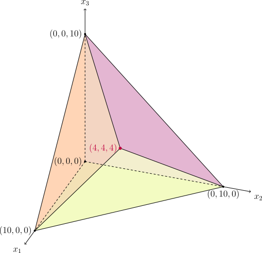
The aforementioned solving process, from a geometric perspective, corresponds to the following path among the vertices of the polyhedron:

\[ (0,0,0) \rightarrow (0,0,10) \rightarrow (10,0,0) \rightarrow (4,4,4). \]

Implementation Details

Using the simplex tableau, we can already solve many linear programming problems. However, for the most general cases, there are still many details in the simplex method worth exploring in depth.

Slack Form

The method to convert a general-form linear programming problem to standard form has been discussed. However, to facilitate solving using the simplex method, we also need to ensure that the coefficient matrix \( A \) is full rank. Although the method of first converting to standard form and then eliminating linearly dependent constraints is feasible, for simplicity, the following strategy is usually adopted:

Convert the linear programming problem to inequality form, i.e., the form \( \min\{c^Tx : Ax \le b,~ x \ge 0\} \);
By adding slack variables \( s \), transform the problem to standard form: \( \min\{c^Tx : Ax + s = b,~ x\ge 0,~ s \ge 0\} \).

The advantage of this approach is that the resulting coefficient matrix \( (A,I) \) in standard form is always full rank, and there always exists a (not necessarily feasible) basic solution \( (x,s)=(0,b) \). This special standard form is also called the slack form.

Initial Basic Feasible Solution

The simplex method described earlier always assumes that a basic feasible solution is known. Sometimes, it is easy to find a basic feasible solution. For example, if \( b\ge 0 \) in the slack form above, then \( (x,s)=(0,b) \) is a basic feasible solution. This is the situation encountered in the numerical example earlier.

For the general case, the two-phase method can be used. In the two-phase method, we perform the simplex method twice. The first phase solves a feasibility linear programming problem to obtain a basic feasible solution for the original problem. The second phase starts from this basic feasible solution and applies the simplex method to solve the original problem.

Suppose we have a problem in standard form \( \min\{c^Tx : Ax = b \ge 0,~ x\ge 0\} \). In the first phase, we solve the problem

\[ \min\{1^Tx_a : Ax + x_a = b,~ x\ge 0,~ s\ge 0\}. \]

This is essentially a feasibility linear programming problem, where the newly added variables \( x_a \) are called artificial variables. It always has a basic feasible solution \( (x,x_a)=(0,b) \), so the simplex method can be applied directly. If the optimal value of this problem is strictly greater than \( 0 \), then there does not exist \( x\ge 0 \) such that \( Ax=b \), meaning the original problem is infeasible. If the optimal value of this problem equals \( 0 \), then in its optimal solution, the artificial variables must be zero. If some artificial variables are still basic variables, we can pivot them out through several pivots. Finally, when all artificial variables are non-basic variables, the basic solution obtained in the first phase can be used as the initial basic feasible solution for the second phase.

First-Phase Implementation Without Explicitly Introducing Artificial Variables

When implementing the first phase, it is not necessary to explicitly introduce artificial variables. For any initially chosen basis \( B \), we have

\[ x_B + A_B^{-1}A_Nx_N = A_B^{-1}b. \]

If \( (A_B^{-1}b)_j\ge 0 \), then no artificial variable is needed; otherwise, we need to additionally introduce an artificial variable \( x^{-}_{B_j} \), i.e.,

\[ x_{B_j} - x^-_{B_j} + (A_B^{-1}A_N)_{(j)}x_N = (A_B^{-1}b)_j. \]

Let the index set \( L:=\{j:(A_B^{-1}b)_j<0\} \). Then the simplex tableau for the first phase is obtained by applying several elementary row transformations to the following simplex tableau:

\[ \begin{array}{|r|c|cccc|} \hline & & x_N & x_{B_{\sim L}} & x_{B_L} &x_{B_{L}}^- \\ \hline & 0 & 0^T & 0^T & 0^T & 1^T \\ \hline x_{B_{\sim L}}= & (A_B^{-1}b)_{\sim L} & (A_B^{-1}A_N)_{(\sim L)} & I & O & O \\ x_{B_{L}}^-= & (A_B^{-1}b)_L & (A_B^{-1}A_N)_{(L)} & O & I & -I \\ \hline \end{array} \]

Similar to simplifying the simplex tableau to the condensed simplex tableau, we can appropriately simplify it: (multiply row \( x_{B_{L}}^- \) by \( 1^T \) and add it to row \( 0 \), then omit the last three columns)

\[ \begin{array}{|r|c|cccc|} \hline & & x_N \\ \hline & 1^Tb_L & 1^T(A_B^{-1}A_N)_L \\ \hline x_{B_{\sim L}}= & (A_B^{-1}b)_{\sim L} & (A_B^{-1}A_N)_{(\sim L)} \\ -x_{B_{L}}= & (A_B^{-1}b)_L & (A_B^{-1}A_N)_L \\ \hline \end{array} \]

This is largely consistent with the normal condensed simplex tableau, except that the variables in the last row are marked with a negative sign, indicating that this row still contains artificial variables, meaning the original slack variables are still infeasible. Using this tableau, the pivoting process is as follows:

If \( L=\varnothing \), the algorithm terminates.
Otherwise, select an entering variable \( x_{N_i} \) based on the condition that the reduced cost in row \( 0 \) is negative. If none exists, then the original problem is infeasible, and the algorithm terminates.
Then select a leaving variable \( x_{B_j} \) based on column \( i \). Still use the minimum ratio test, but require that both the current feasible variables remain feasible and the current infeasible variables remain infeasible, i.e., select

\[ \arg\min_{j}\left\{\dfrac{(\tilde T_B)_{j0}}{(\tilde T_B)_{ji}}:(j\notin L\land(\tilde T_B)_{ji}>0)\lor(j\in L\land(\tilde T_B)_{ji}<0)\right\} \]

as the row index of the leaving variable. If there are multiple such leaving variables, prioritize infeasible leaving variables.
Let \( x_{N_i} \) enter and \( x_{B_j} \) leave, and update the simplex tableau.
If \( j\in L \), then remove \( j \) from \( L \) (i.e., remove the negative sign mark from that row), and add \( 1 \) to \( (\tilde T_B)_{0i} \).

The reason we can omit the columns corresponding to artificial variables is that if they are still basic variables, their corresponding columns are \( e_j \), which need not be recorded; and if they are no longer basic variables, they will not enter the basis again, so they also need not be recorded. When an artificial variable leaves the basis, it needs to be replaced by the corresponding non-artificial variable, which is the purpose of the last step in the above process.

A reference implementation is as follows:

Reference Implementation

// First phase: find an initial BFS.
// Return false if no feasible solution.
bool initialize() {
  int neg_count = 0;
  for (int j = 0; j < m; ++j) {
    if (tab[n][j] < -eps) {
      for (int i = 0; i <= n; ++i) {
        tab[i][m + 1] += tab[i][j];
      }
      B[j] = ~B[j];
      ++neg_count;
    }
  }
  while (neg_count) {
    int x = -1;
    long double mi = -eps;
    for (int i = 0; i < n; ++i) {
      if (tab[i][m + 1] < mi) {
        x = i;
        mi = tab[i][m + 1];
      }
    }
    if (x == -1) return false;
    int y = -1;
    mi = INFINITY;
    for (int j = 0; j < m; ++j) {
      if ((B[j] < 0 && tab[x][j] < -eps) || (B[j] >= 0 && tab[x][j] > eps)) {
        auto tmp = tab[n][j] / tab[x][j] + (B[j] < 0 ? -eps : eps);
        if (tmp < mi) {
          y = j;
          mi = tmp;
        }
      }
    }
    if (B[y] < 0) {
      --neg_count;
      B[y] = ~B[y];
      pivot(x, y);
      tab[x][m + 1] += 1;
    } else {
      pivot(x, y);
    }
  }
  return true;
}

Before starting the first phase, an extra row is added to record the objective function of the first phase. When pivoting, pivot the entire tableau, including the objective function of the second phase. This way, when the first phase completes, the objective function of the second phase is also updated accordingly, and we can directly start the simplex method of the second phase.

The two-phase method can also be implemented with a single simplex method. By taking a sufficiently large positive number \( M \), we can directly solve the problem

\[ \min\{c^Tx + M1^Tx_a : Ax + x_a = b,~ x\ge 0,~ s\ge 0\} \]

to obtain the optimal solution to the original problem. In implementation, \( M \) is not assigned a specific numerical value but is treated as an unknown sufficiently large positive number during operations. This method is called the big \( M \) method.

The Practical Efficiency of the Naive Algorithm is Exponential

Since the slack form always has an initial basic solution, though not necessarily feasible, a simple idea to find an initial basic feasible solution is to start from an infeasible basic solution and repeatedly use pivoting operations to pivot out infeasible basic variables, selecting non-basic variables corresponding to columns with negative numbers in the same row to enter, until all basic variables are non-negative. A reference implementation is as follows:

Reference Implementation

// First phase: find an initial BFS.
// Return false if no feasible solution.
bool initialize() {
  while (true) {
    int y = -1;
    long double mi = -eps;
    for (int j = 0; j < m; ++j) {
      if (tab[n][j] <= mi) {
        y = j;
        mi = tab[n][j];
      }
    }
    // No row with a negative basic variable => Feasible.
    if (y == -1) break;
    int x = -1;
    for (int i = 0; i < n; ++i) {
      if (tab[i][y] < -eps && (x == -1 || N[i] > N[x])) {
        x = i;
      }
    }
    // No column with a negative entry => Infeasible.
    if (x == -1) return false;
    pivot(x, y);
  }
  return true;
}

Although this is simple, compared to the two-phase method, it lacks an objective function describing the degree of infeasibility of the current basis, so there is no clear direction for improvement. Actual tests show that compared to the two-phase method or the big \( M \) method, which typically require \( O(m) \) pivots, this naive algorithm usually requires \( O(2^m) \) pivots, and when \( n,m \) are large, it easily falls into cycles. Although the constant in the number of pivots for the naive algorithm is small, it is only suitable for situations where \( n,m<50 \).

Pivot Rules

When pivoting, if there are multiple possible entering or leaving variables, pivot rules are needed to decide which variable to enter or leave. Using the simplex tableau, all rules discussed in this section can find entering and leaving variables in \( O(mn) \) time, so the time complexity of a single pivot remains \( O(mn) \).

The choice of entering variable often determines the number of pivots before algorithm termination. Common rules include:

Choose the first entering variable found;
Choose the entering variable with the smallest index; (part of Bland's rule)
Choose the entering variable with the largest absolute reduced cost (i.e., \( |c_i| \)); (Dantzig's rule)
Choose the entering variable that yields the largest improvement in the objective function per pivot (i.e., \( |c_i|\theta_i \));
Choose the entering variable corresponding to the steepest edge, i.e., the one that yields the largest improvement in the objective function per unit length moved along the edge (i.e., \( |c_i|/\|A_B^{-1}A_i\| \));
Randomly choose an entering variable.

In practice, the steepest edge rule is the most efficient². It is generally believed that appropriate pivot rules can obtain the optimal solution for most problems in roughly \( 2m \) pivots. However, for all currently known pivot rules, there exist specially constructed examples³ that can force the number of pivots to be exponential. This is precisely why the simplex method performs quite well in practice but has exponential worst-case theoretical complexity.

The choice of leaving variable often determines whether the algorithm will cycle. If there are multiple basic feasible solutions with the same optimal value, the algorithm may cycle among these basic feasible solutions. Such situations are not common, so many simplex method implementations do not specify a rule for selecting the leaving variable. There are two common rules to avoid cycling:

Bland's rule: Always choose the entering and leaving variables with the smallest indices.
Lexicographic rule: Always choose the row index \( j \) corresponding to the leaving variable \( x_{B_j} \) such that \( (A_B^{-1}A_i)_j>0 \) and

\[ \left(\dfrac{(A_B^{-1}b)_j}{(A_B^{-1}A_i)_j},\dfrac{(A_B^{-1})_{j1}}{(A_B^{-1}A_i)_j},\cdots,\dfrac{(A_B^{-1})_{jm}}{(A_B^{-1}A_i)_j}\right) \]

is lexicographically smallest. The choice of entering variable is not important.

Note that if the linear programming problem is in slack form, these quantities can be directly found from the simplex tableau \( T_B \) in the form described earlier; otherwise, after finding an initial basic solution (not necessarily feasible), we can use the coefficients of the columns corresponding to the basic variables in these initial bases (keeping the order fixed) as the coefficients of \( A_B^{-1} \).

Bland's rule is very inefficient because the rule itself uses the same method for selecting entering and leaving variables, which easily causes the same variable to repeatedly enter and leave the basis. Comparatively, the lexicographic rule is more practical. The lexicographic rule is equivalent to perturbing the parameters of the linear programming problem slightly⁴, ensuring that there are no basic feasible solutions with the same optimal value, thus eliminating the possibility of cycling.

Reference Implementation

This section provides a reference implementation of a two-phase simplex method based on the condensed simplex tableau.

Luogu P13337【Template】Linear Programming

#include <algorithm>
#include <climits>
#include <cmath>
#include <iomanip>
#include <iostream>
#include <numeric>
#include <vector>

int m, n;  // Number of constraints and variables.
std::vector<std::vector<long double>>
    tab;                             // Compressed tableau (transposed) with
                                     // first-phase objective attached.
std::vector<int> B, N;               // Basic and nonbasic variables.
constexpr long double eps = 1e-12l;  // Precision.

// Pivot on (N[x], B[y]).
void pivot(int x, int y) {
  std::swap(N[x], B[y]);
  long double v = -1 / tab[x][y];
  for (int j = 0; j <= m + 1; ++j) {
    tab[x][j] = j == y ? -v : v * tab[x][j];
  }
  for (int i = 0; i <= n; ++i) {
    if (i == x) continue;
    v = tab[i][y];
    tab[i][y] = 0;
    for (int j = 0; j <= m + 1; ++j) {
      tab[i][j] += v * tab[x][j];
    }
  }
}

// First phase: find an initial BFS.
// Return false if no feasible solution.
bool initialize() {
  int neg_count = 0;
  for (int j = 0; j < m; ++j) {
    if (tab[n][j] < -eps) {
      for (int i = 0; i <= n; ++i) {
        tab[i][m + 1] += tab[i][j];
      }
      B[j] = ~B[j];
      ++neg_count;
    }
  }
  while (neg_count) {
    int x = -1;
    long double mi = -eps;
    for (int i = 0; i < n; ++i) {
      if (tab[i][m + 1] < mi) {
        x = i;
        mi = tab[i][m + 1];
      }
    }
    if (x == -1) return false;
    int y = -1;
    mi = INFINITY;
    for (int j = 0; j < m; ++j) {
      if ((B[j] < 0 && tab[x][j] < -eps) || (B[j] >= 0 && tab[x][j] > eps)) {
        auto tmp = tab[n][j] / tab[x][j] + (B[j] < 0 ? -eps : eps);
        if (tmp < mi) {
          y = j;
          mi = tmp;
        }
      }
    }
    if (B[y] < 0) {
      --neg_count;
      B[y] = ~B[y];
      pivot(x, y);
      tab[x][m + 1] += 1;
    } else {
      pivot(x, y);
    }
  }
  return true;
}

// Second phase: find an optimal BFS.
// Return false if the problem is unbounded.
bool simplex() {
  while (true) {
    int x = -1;
    long double mi = -eps;
    for (int i = 0; i < n; ++i) {
      if (tab[i][m] < mi) {
        x = i;
        mi = tab[i][m];
      }
    }
    // No column with a negative reduced cost => Optimal.
    if (x == -1) break;
    int y = -1;
    mi = INFINITY;
    for (int j = 0; j < m; ++j) {
      if (tab[x][j] <= eps) continue;
      if (tab[n][j] / tab[x][j] < mi) {
        y = j;
        mi = tab[n][j] / tab[x][j];
      }
    }
    // No row with a positive ratio => Unbounded.
    if (y == -1) return false;
    pivot(x, y);
  }
  return true;
}

int solve() {
  B.resize(m);
  N.resize(n);
  std::iota(B.begin(), B.end(), n);
  std::iota(N.begin(), N.end(), 0);
  return initialize() ? (simplex() ? 0 : 1) : -1;
}

int main() {
  std::ios::sync_with_stdio(false), std::cin.tie(nullptr);
  std::cout << std::fixed << std::setprecision(8);
  std::cin >> n >> m;
  tab.assign(n + 1, std::vector<long double>(m + 2));
  for (int i = 0; i < n; ++i) {
    std::cin >> tab[i][m];
    tab[i][m] = -tab[i][m];
  }
  for (int j = 0; j < m; ++j) {
    for (int i = 0; i <= n; ++i) {
      std::cin >> tab[i][j];
    }
  }
  switch (solve()) {
    case -1:
      std::cout << "Infeasible" << std::endl;
      break;
    case 1:
      std::cout << "Unbounded" << std::endl;
      break;
    case 0: {
      std::cout << tab[n][m] << std::endl;
      std::vector<long double> x(n);
      for (int j = 0; j < m; ++j) {
        if (B[j] < n) x[B[j]] = tab[n][j];
      }
      for (int i = 0; i < n; ++i) {
        std::cout << x[i] << ' ';
      }
      std::cout << std::endl;
      break;
    }
  }
  return 0;
}

Example Problems

「NOI2008」Volunteer Recruitment

A total of \( n \) days of activities require volunteer recruitment, where at least \( b_i \) volunteers are needed on day \( i \). There are \( m \) types of volunteers, where the \( j \)-th type can serve during the continuous interval \( [l_j,r_j] \), and the unit recruitment cost is \( c_i \). Find the optimal recruitment plan to minimize the cost of recruiting volunteers.

Solution

Let \( x_j \) be the number of volunteers of type \( j \) recruited. Then, we can formulate the linear programming problem as

\[ \begin{align*} \max_{x}\; & \sum_{j=1}^mc_jx_j \\ \text{subject to }& \sum_{i=1}^n a_{ij}x_j \ge b_i,~i=1,\cdots,n,\\ & x_j\ge 0,~j=1,\cdots,m. \end{align*} \]

where the coefficients

\[ a_{ij} = \begin{cases} 1,& l_j\le i\le r_j,\\ 0,& \text{otherwise.} \end{cases} \]

The original problem does not have an obvious initial feasible solution. Therefore, consider its dual problem:

\[ \begin{align*} \min_{y}\; & \sum_{i=1}^n b_iy_i \\ \text{subject to } & \sum_{j=1}^na_{ij}y_i \le c_j,~j=1,\cdots,m,\\ & y_i\ge 0,~i=1,\cdots,n. \end{align*} \]

By adding slack variables, it is easy to obtain an initial feasible solution, allowing us to skip the first phase and solve directly using the simplex method. According to duality theory, the solution obtained is the solution to the original problem.

#include <cmath>
#include <cstring>
#include <iostream>
using namespace std;
constexpr int M = 10005, N = 1005, INF = 1e9;

int n, m;
double a[M][N], b[M], c[N], v;

void pivot(int l, int e) {  // Pivot operation function
  b[l] /= a[l][e];
  for (int j = 1; j <= n; j++)
    if (j != e) a[l][j] /= a[l][e];
  a[l][e] = 1 / a[l][e];

  for (int i = 1; i <= m; i++)
    if (i != l && fabs(a[i][e]) > 0) {
      b[i] -= a[i][e] * b[l];
      for (int j = 1; j <= n; j++)
        if (j != e) a[i][j] -= a[i][e] * a[l][j];
      a[i][e] = -a[i][e] * a[l][e];
    }

  v += c[e] * b[l];
  for (int j = 1; j <= n; j++)
    if (j != e) c[j] -= c[e] * a[l][j];
  c[e] = -c[e] * a[l][e];

  // swap(B[l],N[e])
}

double simplex() {
  while (true) {
    int e = 0, l = 0;
    for (e = 1; e <= n; e++)
      if (c[e] > (double)0) break;
    if (e == n + 1) return v;  // v is the optimal solution at this point
    double mn = INF;
    for (int i = 1; i <= m; i++) {
      if (a[i][e] > (double)0 && mn > b[i] / a[i][e]) {
        mn = b[i] / a[i][e];  // Find the l that imposes the tightest constraint on this e
        l = i;
      }
    }
    if (mn == INF) return INF;  // unbounded
    pivot(l, e);                // Pivot on l,e
  }
}

int main() {
  cin.tie(nullptr)->sync_with_stdio(false);
  cin >> n >> m;
  for (int i = 1; i <= n; i++) cin >> c[i];
  for (int i = 1; i <= m; i++) {
    int s, t;
    cin >> s >> t;
    for (int j = s; j <= t; j++) a[i][j] = 1;  // Indicates that the i-th volunteer can serve at time j
    cin >> b[i];
  }
  cout << (int)(simplex() + 0.5);
}

Exercises

References

Linear Programming Simplex Method【Detailed Explanation + Diagram】
2016 National Training Team Papers
Introduction to Algorithms
Matoušek, Jiří, and Bernd Gärtner. Understanding and using linear programming. Vol. 1. Berlin: Springer, 2007.
Inayatullah, Syed, Nasir Touheed, and Muhammad Imtiaz. "A streamlined artificial variable free version of simplex method." PloS one 10, no. 3 (2015): e0116156.
Floudas, Christodoulos A., and Panos M. Pardalos, eds. Encyclopedia of optimization. Springer Science & Business Media, 2008.

In principle, since all vectors are column vectors by default, \( (x_B,x_N) \) should be written as \( (x_B^T,x_N^T)^T \). But to simplify notation, all similar cases in this article are directly written as \( (x_B,x_N) \), omitting the transpose symbol. ↩
Test results can be found in Forrest, John J., and Donald Goldfarb. "Steepest-edge simplex algorithms for linear programming." Mathematical programming 57, no. 1 (1992): 341-374. ↩
A classic counterexample can be found in Klee, Victor, and George J. Minty. "How good is the simplex algorithm." Inequalities 3, no. 3 (1972): 159-175. ↩
Detailed explanation can be found in this lecture note. ↩

本页面最近更新：，更新历史
发现错误？想一起完善？在 GitHub 上编辑此页！
本页面贡献者：OI-wiki
本页面的全部内容在 CC BY-SA 4.0 和 SATA 协议之条款下提供，附加条款亦可能应用