Sparse Table
Definition
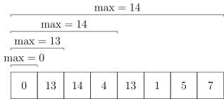
The Sparse Table (ST table) is a data structure used to solve repeatedly contributive problems.
What is a repeatedly contributive problem?
A repeatedly contributive problem refers to an operation \(\operatorname{opt}\) that satisfies \(x\operatorname{opt} x=x\). Then the corresponding interval query is a repeatedly contributive problem. For example, maximum satisfies \(\max(x,x)=x\), GCD satisfies \(\operatorname{gcd}(x,x)=x\), so RMQ and interval GCD are repeatedly contributive problems. Interval sum does not have this property: if the preprocessed intervals overlap when computing the interval sum, the overlapping part will be calculated twice, which is undesirable. Additionally, \(\operatorname{opt}\) must also satisfy associativity to be solvable using an ST table.
What is RMQ?
RMQ stands for Range Maximum/Minimum Query. There are many methods to solve RMQ problems; refer to RMQ Topic.
Introduction
Luogu P3865【Template】ST Table & RMQ Problem
Given \(n\) (\(1\le n\le 10^5\)) integers and \(m\) (\(1\le m\le 2\times 10^6\)) queries, for each query, you need to answer the maximum value in the interval \([l,r]\).
Consider a brute-force approach: scan the interval \([l,r]\) each time to find the maximum.
Obviously, this algorithm will time out.
ST Table
The ST table is based on the idea of binary lifting. It can achieve \(\Theta(n\log n)\) preprocessing and \(\Theta(1)\) answering per query. However, it does not support modification operations.
Based on the binary lifting idea, consider how to compute the interval maximum. If we follow the usual binary lifting process, jumping \(2^i\) steps each time, the query complexity would still be \(\Theta(\log n)\), which is not better than a segment tree, and the preprocessing step is even slower.
We note that \(\max(x,x)=x\), meaning the interval maximum is a problem with the "repeatedly contributive" property. Even if the preprocessed intervals used for solving overlap, as long as their union is the target interval, the final computed answer will be correct.
Manually simulating this reveals that we can cover the query interval using at most two preprocessed intervals. This means the query time complexity can be reduced to \(\Theta(1)\), which is very effective for problems with many queries.
The specific implementation is as follows:
Let \(f(i,j)\) denote the maximum value of the interval \([i,i+2^j-1]\).
Clearly, \(f(i,0)=a_i\).
According to the definition, the second dimension corresponds to "jumping \(2^j-1\) steps" in binary lifting. Following the binary lifting idea, the state transition equation is: \(f(i,j)=\max(f(i,j-1),f(i+2^{j-1},j-1))\).
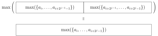
The above is the preprocessing part. For queries, it can be simply implemented as follows:
For each query \([l,r]\), we split it into two parts: \([l,l+2^s-1]\) and \([r-2^s+1,r]\), where \(s=\left\lfloor\log_2(r-l+1)\right\rfloor\). The maximum of the results from these two parts is the answer.
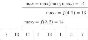
Based on the earlier argument about "repeatedly contributive problems," since the maximum is a "repeatedly contributive problem," overlap does not affect the interval maximum. Moreover, these two intervals completely cover \([l,r]\), ensuring the correctness of the answer.
Luogu P3865【Template】ST Table & RMQ Problem Reference Implementation
1 2 3 4 5 6 7 8 9 10 11 12 13 14 15 16 17 18 19 20 21 22 23 24 25 26 27 28 29 30 31 32 | |
1 2 3 4 5 6 7 8 9 10 11 12 13 14 15 16 17 18 19 20 21 22 23 24 25 26 27 28 29 30 31 32 33 34 35 36 37 38 39 40 41 42 43 44 45 46 47 48 49 50 51 52 53 54 55 56 57 58 59 60 | |
1 2 3 4 5 6 7 8 9 10 11 12 13 14 15 16 17 18 19 20 21 22 23 24 25 26 27 28 29 30 31 32 33 34 35 36 37 | |
Notes
-
Input and output data are usually large; it is recommended to enable input/output optimization.
-
When preprocessing the ST table, we typically need to create an array with one dimension of size \(\log n\) and the other of size \(n\). In this case, prioritize making the dimension of size \(\log n\) the first dimension to improve cache locality.
-
Recalculating the logarithm function each time using std::log is not worthwhile. It is recommended to use built-in functions like
__builtin_clzor__lgfor computation. If these built-in functions are unavailable, you can also precompute the logarithm function values. The preprocessing method is as follows:
ST Table Maintaining Other Information
Besides RMQ, there are other "repeatedly contributive problems," such as "interval bitwise AND," "interval bitwise OR," and "interval GCD." The ST table can efficiently solve these.
Note that for "interval GCD," the query complexity of the ST table is not better than that of a segment tree (let the value range be \(w\); the ST table's query complexity is \(\Theta(\log w)\), while the segment tree's is \(\Theta(\log n+\log w)\), and the value range is generally larger than \(n\)). However, the preprocessing complexity of the ST table is not worse than that of a segment tree, and the programming complexity of the ST table is much simpler than that of a segment tree.
Analyzing further, "repeatedly contributive problems" generally involve some component similar to RMQ. For example, "interval bitwise AND" takes the minimum for each bit, while "interval GCD" takes the minimum exponent for each prime factor.
Summary
The ST table can effectively maintain interval information that is "repeatedly contributive" (and also associative), with low time complexity and relatively small code size compared to other algorithms. However, the ST table can maintain very limited information, does not extend well, and does not support modification operations.
Exercises
Appendix: Time Complexity Analysis of ST Table for Interval GCD
During the algorithm's execution, there may be \(\Theta(\log n)\) iterations. Each iteration may use the GCD function recursively. Let the value range be \(w\); the worst-case time complexity of the GCD function is \(\Omega(\log w)\). Thus, the total time complexity appears to be \(O(n\log n\log w)\).
However, during the GCD process, each recursion (except the last) reduces at least one number in the sequence by half. The maximum number of times a number in the sequence can be halved is \(\log_2 (w^n)=\Theta(n\log w)\). Therefore, the recursive part of GCD runs at most \(O(n\log w)\) times. Adding the loop part (and the last recursion) of \(\Theta(n\log n)\), the final time complexity is \(O(n(\log w+\log n))\). Since data can be constructed to make the time complexity \(\Omega(n(\log w+\log n))\), the final time complexity is \(\Theta(n(\log w+\log n))\).
The query part's time complexity is easy to analyze. Considering the worst case, where each query asks for the worst pair, the time complexity is \(\Theta(\log w)\). Therefore, the time complexity for the ST table maintaining "interval GCD" is preprocessing \(\Theta(n(\log n+\log w))\) and single query \(\Theta(\log w)\).
The corresponding operations for a segment tree are preprocessing \(\Theta(n\log w)\) and single query \(\Theta(\log n+\log w)\).
This is not a rigorous mathematical proof; a more rigorous one is provided below:
More Rigorous Proof
Understanding this section may require knowledge of "potential analysis" in time complexity.
First, analyze the time complexity of the preprocessing part:
Define the "sequence under consideration" as the sequence in the current layer's loop during ST table preprocessing. For example, the zeroth layer's sequence is the original sequence, the first layer's sequence is the sequence after one iteration of the zeroth layer, i.e., st[1..n][1], denoted as \(A\).
The potential function is defined as the base-2 logarithm of the product of all numbers in the "sequence under consideration." That is: \(\Phi(A)=\log_2\left(\prod\limits_{i=1}^n A_i\right)\).
In one iteration, the time spent is equivalent to the sum of the time spent in the iteration loop and the time spent on GCD. The time spent on GCD varies. The shortest may be only two or even one recursion, while the longest may be \(O(\log w)\) recursions. However, during the GCD process, except for the first and last layers, each recursion reduces at least one result in the "sequence under consideration" by half. That is, \(\Phi(A)\) decreases by at least \(1\), and the time used for that layer of recursion can be amortized by the potential function.
Additionally, we see that the initial value of \(\Phi(A)\) is at most \(\log_2 (w^n)=\Theta(n\log w)\), and \(\Phi(A)\) does not increase. Therefore, the time complexity of the ST table preprocessing part is \(O(n(\log w+\log n))\).
本页面最近更新:,更新历史
发现错误?想一起完善? 在 GitHub 上编辑此页!
本页面贡献者:OI-wiki
本页面的全部内容在 CC BY-SA 4.0 和 SATA 协议之条款下提供,附加条款亦可能应用