K-D Tree
k-D Tree (KDT, k-Dimension Tree) is a data structure that can efficiently process \(k\)-dimensional spatial information.
When the number of nodes \(n\) is much larger than \(2^k\), k-D Tree performs well in terms of time efficiency.
In algorithmic contest problems, typically \(k=2\). In the time complexity analysis on this page, \(k\) is considered a constant.
Building the Tree
A k-D Tree has the structure of a binary search tree, where each node corresponds to a point in \(k\)-dimensional space. All points in each subtree lie within a \(k\)-dimensional hyperrectangle, and all points within that hyperrectangle are also in that subtree.
Suppose we know the coordinates of \(n\) distinct points in \(k\)-dimensional space and want to build a k-D Tree from them. The steps are as follows:
- If the current hyperrectangle contains only one point, return that point.
- Choose a dimension and split the current hyperrectangle into two hyperrectangles along that dimension.
- Select a split point: choose a point along the selected dimension; points with values less than this point go into one hyperrectangle (left subtree), and the rest go into the other hyperrectangle (right subtree).
- Use the selected point as the root of this subtree, recursively build left and right subtrees for the two hyperrectangles, and maintain subtree information.
For easier understanding, let's take an example with \(k=2\).
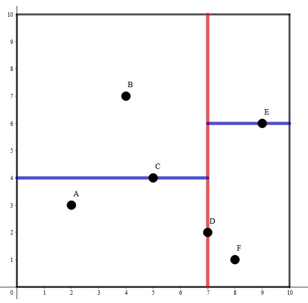
The resulting k-D Tree might look like this:
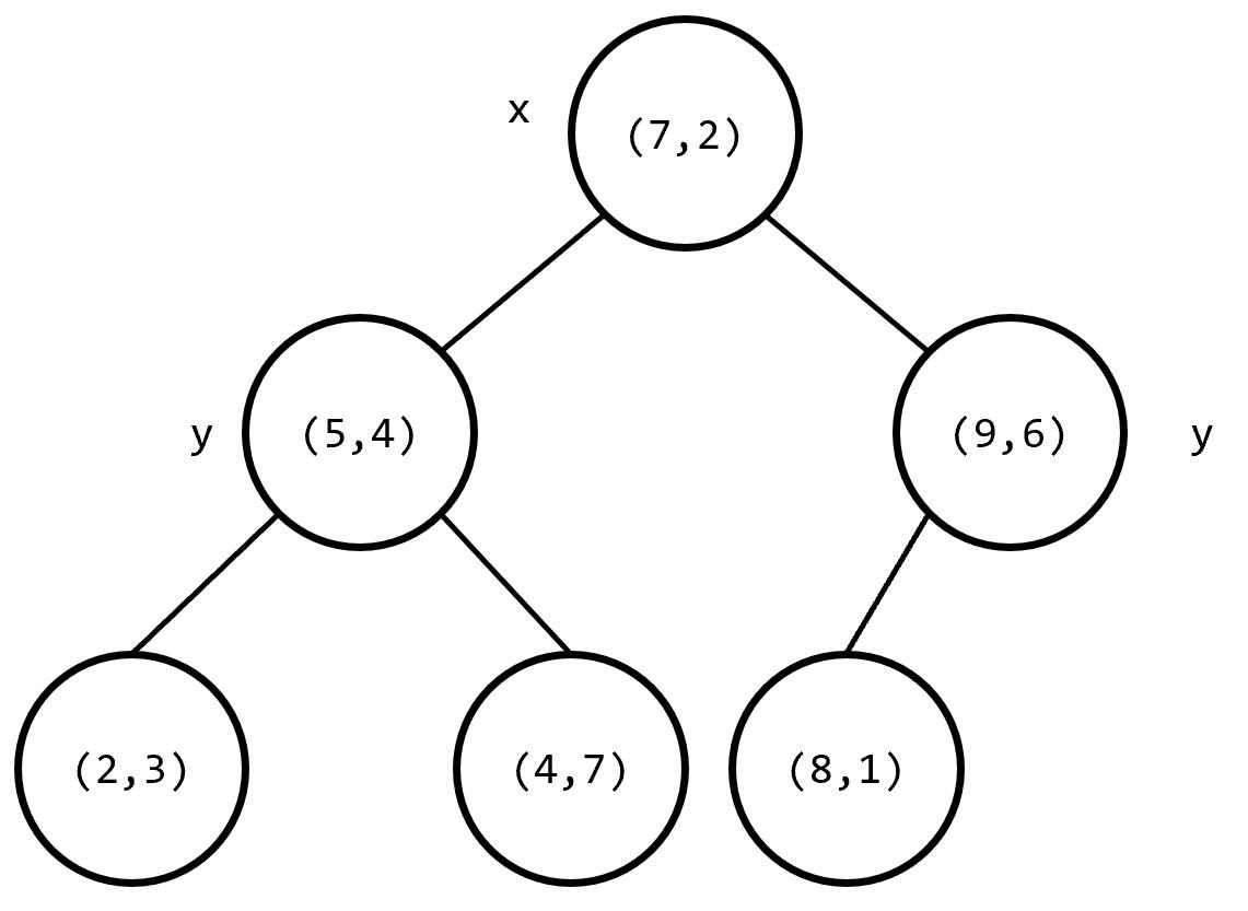
Here, the coordinates on each tree node are the coordinates of the chosen split point, and the \(x\) or \(y\) beside non-leaf nodes indicates the chosen splitting dimension.
This naive approach does not guarantee good complexity. For steps 2 and 3, we propose two optimizations:
- Alternate among the \(k\) dimensions to ensure that every dimension is split within any consecutive \(k\) layers.
- Each time, choose the median along the selected dimension as the split point, ensuring that the left and right subtrees are as balanced as possible.
With optimization 2, the height of the constructed k-D Tree is at most \(\log n+O(1)\).
Now, the bottleneck in building a k-D Tree is quickly selecting the median along a dimension and placing values less than the median to its left and the rest to its right. If we sort the dimension each time using sort, the time complexity would be \(O(n\log^2 n)\). In fact, finding the median among \(n\) elements and placing it in its correct sorted position can be done in \(O(n)\).
Recall the idea of quicksort. Each time we pick a pivot, place elements smaller than the pivot to its left and larger ones to its right, ensuring the pivot is in its correct sorted position, then recursively sort the left and right parts. The expected complexity is \(O(n\log n)\). However, since k-D Tree only requires the median to be in its correct sorted position, we only need to recursively sort the side containing the median. It can be proven that the expected complexity of this is \(O(n)\). In the algorithm library, the function nth_element() achieves the same functionality. To find the value that would be at position s[mid] if the range [s[l], s[r]] were sorted according to comparator cmp, and ensure all elements before s[mid] are less than s[mid] and all after are greater, simply write nth_element(s+l, s+mid, s+r+1, cmp).
With this idea, building a k-D Tree can be done in \(O(n\log n)\) time.
Operations in High-Dimensional Space
When querying some information about all points within a high-dimensional rectangular region, we record the minimum and maximum coordinates in each dimension for each node's subtree. If the rectangle corresponding to the current subtree does not intersect the query rectangle, we do not search its subtrees further. If the current subtree's rectangle is completely contained within the query rectangle, we return the sum of weights of all points in that subtree. Otherwise, we check if the current point lies within the query rectangle, update the answer, and recursively search the left and right subtrees.
Implementation
1 2 3 4 5 6 7 8 9 10 11 12 13 | |
Complexity Analysis
Consider the two-dimensional case. When querying rectangle \(R\), we classify nodes in the k-D Tree into three categories:
- No intersection with \(R\).
- Completely contained within \(R\).
- Partially overlapping with \(R\).
Clearly, the complexity of a single query is determined by the number of type 3 nodes. Note that the rectangles of type 3 nodes either completely contain \(R\) or are disjoint from \(R\). The former obviously has only \(O(h)=O(\log n)\) nodes. Now we analyze the number of the latter.
First, we can offset all edges of the rectangle by \(\epsilon\) so that the query rectangle does not pass through any existing point. This does not affect the set of points covered by the query.
Notice that for disjoint type 3 nodes, one edge of \(R\) must pass through their rectangle. Therefore, we only need to count how many rectangles each edge of \(R\) passes through, i.e., the maximum number of point rectangles any axis-aligned line segment can intersect.
Consider a node \(u\) with four grandchildren, where each split from \(u\) to a grandchild divides along two dimensions. Observation shows that dividing a rectangle into four subrectangles in this way, any axis-aligned line segment can intersect at most two regions. That is, starting from \(u\), a query can descend into at most two grandchildren while still having type 3 nodes (if the segment exactly coincides with a split boundary, it might be more, but our offset operation eliminates this case).
Since during construction, each point is the median of its entire subtree along the current splitting dimension, the subtree size must halve. Let the subtree size of \(u\) be \(n\). We can write the recurrence:
By the Master Theorem, \(T(n)=O(\sqrt{n})\).
Generalizing the recurrence to \(k\) dimensions, i.e., \(T(n)=2^{k-1}T(n/2^k)+O(1)\), we get \(T(n)=O(n^{1-\frac1k})\) (treating \(k\) as a constant).
Insertion/Deletion
If the \(k\)-dimensional point set is dynamic, i.e., points may be inserted or deleted, the balance of the k-D Tree cannot be guaranteed. Due to the construction of k-D Tree, rotations are not supported, and random priorities similar to FHQ Treap cannot guarantee complexity. Two common maintenance methods are described below.
Note
Many contestants use the Scapegoat Tree structure for maintenance. However, note that in the previous complexity analysis, we required the child subtree sizes to strictly halve, i.e., the tree height must be exactly \(\log n+O(1)\). Scapegoat Tree only guarantees tree height \(O(\log n)\), so query complexity cannot be guaranteed.
Square Root Rebuilding
When inserting, store the points to be inserted and rebuild every \(B\) insertions.
For deletion, just mark the node as deleted. If stricter requirements are needed, maintain the count of deleted nodes in the tree and rebuild when it reaches \(B\).
Modification complexity is amortized \(O(n\log n/B)\), query complexity is \(O(B+n^{1-\frac1k})\). If the number of modifications and queries are of the same order, then \(B=O(\sqrt{n\log n})\) is optimal (modification \(O(\sqrt{n\log n})\), query \(O(\sqrt{n\log n}+n^{1-\frac1k})\)).
Binary Grouping
Maintain several k-D Trees whose sizes are powers of \(2\), such that their total size sums to \(n\).
When inserting, add a new k-D Tree of size \(1\), then repeatedly merge trees of the same size (by flattening and rebuilding). In implementation, rebuilding can be done only once.
It is easy to see that the sizes of trees to be merged must start from \(2^0\) and be consecutive powers of two. The complexity is similar to binary addition, amortized \(O(n\log^2 n)\) because rebuilding itself has a \(\log\) factor.
When querying, query each tree directly. The complexity is \(O\left(\sum_{i\geq0} (\frac n{2^i})^{1-\frac1k}\right)=O(n^{1-\frac1k})\).
Example Problems
Luogu P4148 Simple Problem
On an \(n\times n\) 2D matrix initially filled with zeros, perform \(q\) operations, each being one of the following:
1 x y A: Add \(A\) to the number at coordinate \((x,y)\).2 x1 y1 x2 y2: Output the sum of numbers within the rectangle with bottom-left corner \((x1,y1)\) and top-right corner \((x2,y2)\) (including boundaries).
Forced online. Memory limit 20M. Ensure the answer and all intermediate values fit within int.
\(1\le n\le 500000 , 1\le q\le 200000\)
The 20M memory limit rules out all tree-of-trees structures, and forced online rules out CDQ divide-and-conquer, leaving k-D Tree as the only option.
Below is reference code using binary grouping.
Reference Code
1 2 3 4 5 6 7 8 9 10 11 12 13 14 15 16 17 18 19 20 21 22 23 24 25 26 27 28 29 30 31 32 33 34 35 36 37 38 39 40 41 42 43 44 45 46 47 48 49 50 51 52 53 54 55 56 57 58 59 60 61 62 63 64 65 66 67 68 69 70 71 72 73 74 75 76 77 78 79 80 81 82 83 84 85 86 87 88 89 90 91 92 93 94 95 96 97 98 99 | |
Neighborhood Queries
Warning
The worst-case time complexity for a single nearest neighbor query using k-D Tree is still \(O(n)\). However, it serves as an excellent "cheating" algorithm. Use with caution. The discussion of neighborhood queries here is only to deepen understanding of the k-D Tree structure.
Example Luogu P1429 Plane Nearest Point Pair (Enhanced)
Given \(n\) points \((x_i,y_i)\) in the plane, find the Euclidean distance between the closest pair of points.
\(2\le n\le 200000 , 0\le x_i,y_i\le 10^9\)
First, build a 2-D Tree for these \(n\) points.
For each node, find the closest point (excluding itself) to compute the answer. A brute-force traversal of all nodes in the 2-D Tree would be \(O(n)\) per query, so pruning is needed. We can maintain the minimum and maximum coordinates in each dimension for all points in a subtree. Suppose the current best distance found is \(ans\). If the minimum distance from the query point to the bounding box containing all points in the subtree is greater than or equal to \(ans\), then there cannot be a better answer in that subtree, so we skip it.
Additionally, a heuristic search can be used: if both children of a node might contain the answer, search the subtree whose bounding box is closer to the query point first. The minimum distance from the query point to the bounding box of a subtree can be considered as the heuristic function for this problem.
Reference Code
1 2 3 4 5 6 7 8 9 10 11 12 13 14 15 16 17 18 19 20 21 22 23 24 25 26 27 28 29 30 31 32 33 34 35 36 37 38 39 40 41 42 43 44 45 46 47 48 49 50 51 52 53 54 55 56 57 58 59 60 61 62 63 64 65 66 67 68 69 70 71 72 73 74 75 76 77 78 79 80 81 82 83 84 85 86 87 88 89 90 91 92 93 94 95 96 97 98 | |
Example 「CQOI2016」K-th Far Point Pair
Given \(n\) points \((x_i,y_i)\) in the plane, find the Euclidean distance of the \(k\)-th farthest unordered point pair.
\(n\le 100000 , 1\le k\le 100 , 0\le x_i,y_i<2^{31}\)
Similar to the previous example, but now we want the \(k\)-th farthest pair instead of the nearest. The heuristic function becomes the maximum distance from the query point to the bounding box of the subtree. Use a min-heap to maintain the current top \(k\) farthest distances found. If a newly found distance is larger than the heap top, pop the heap top and insert the new distance. Similarly, use the heap top distance for pruning.
Since the problem emphasizes unordered point pairs (i.e., swapping the two points gives the same pair), each ordered pair is counted twice. Thus, the input \(k\) should be multiplied by \(2\).
Reference Code
1 2 3 4 5 6 7 8 9 10 11 12 13 14 15 16 17 18 19 20 21 22 23 24 25 26 27 28 29 30 31 32 33 34 35 36 37 38 39 40 41 42 43 44 45 46 47 48 49 50 51 52 53 54 55 56 57 58 59 60 61 62 63 64 65 66 67 68 69 70 71 72 73 74 75 76 77 78 79 80 81 82 83 84 85 86 87 | |
Exercises
「Violet」Angel Doll/SJY Plays Chess
「National Team Training」JZPFAR
「CH Weak Province Contest R2」TATT
本页面最近更新:,更新历史
发现错误?想一起完善? 在 GitHub 上编辑此页!
本页面贡献者:OI-wiki
本页面的全部内容在 CC BY-SA 4.0 和 SATA 协议之条款下提供,附加条款亦可能应用