Tim Sort

This page introduces Timsort, a hybrid, stable sorting algorithm.

Introduction

Timsort was designed by Tim Peters, a core Python developer, in 2002 and implemented in the Python language. It cleverly combines the advantages of insertion sort and merge sort, with precise optimizations for the existing order within datasets. It is particularly well-suited for datasets containing many partially ordered subsequences. Since Python version 2.3, Timsort has been selected as the default sorting algorithm for the Python standard library and has been widely adopted in other programming environments, such as being used for sorting non-primitive object arrays in Java SE 7.

Steps

The core idea of Timsort is to improve sorting efficiency by identifying and utilizing existing order within the dataset. It mainly consists of the following steps:

1. Identify Runs: Scan the array to be sorted to identify consecutive ordered subsequences (Runs).
2. Extend Runs: If the identified Run length is less than MIN_RUN, use insertion sort to extend it.
3. Merge Runs: Timsort maintains a special stack and uses a specific merging strategy to merge the existing Runs in the stack into larger ordered sequences.

Identify Runs

First, Timsort scans the array from left to right to identify consecutive ordered sequences, which are called Runs:

• Ascending Run: If the next element is greater than or equal to the previous element, continue extending the Run.
• Descending Run: If the next element is less than the previous element, continue extending the Run, then reverse this Run to make it ascending.

Extend Runs

To improve sorting efficiency for small-scale data, Timsort introduces a minimum Run length MIN_RUN. Its value is generally calculated dynamically based on the length of the array to be sorted, typically between \(32\) and \(64\).

• If the identified Run length is greater than or equal to MIN_RUN, no additional operation is needed; the Run is directly pushed onto the stack.
• If the identified Run length is less than MIN_RUN, use binary insertion sort to insert subsequent elements into the Run until its length reaches MIN_RUN, then push it onto the stack.

Merge Runs

In Timsort, merge sort is managed and controlled via a stack. The stack holds the identified ordered Runs, and specific merging rules control the merging of Runs in the stack. The goal is to maintain balance and stability of the sequence during merging.

Merging Rules

Timsort is a stable sorting algorithm, meaning elements with equal values maintain their original relative order after sorting. To ensure this, Timsort only merges adjacent, consecutive Runs during merging and does not directly merge non-adjacent Runs. This is because there might be equal elements between non-adjacent Runs, and direct merging could disrupt their relative order.

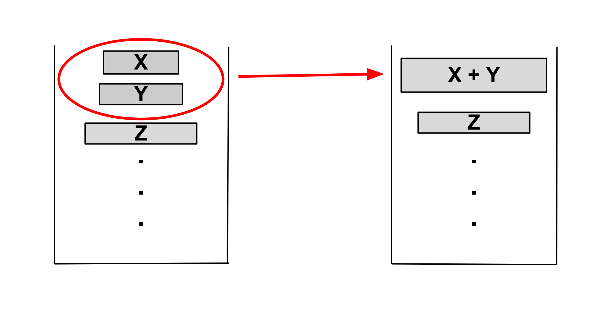
Simultaneously, to ensure merging balance, Timsort introduces specific merging rules. Before each merge operation, the algorithm checks the top three Runs X, Y, and Z on the stack to ensure the following two conditions are met:

• Condition One: len(Z) > len(Y) + len(X)
• Condition Two: len(Y) > len(X)

If the top three Runs on the stack do not satisfy the above conditions, Timsort merges Y with the smaller of X or Z, then checks the conditions again. Once the conditions are satisfied, it continues searching for new Runs, adds them to the stack, and begins the next round of merging.

Merge Optimization

To improve efficiency and reduce space overhead when merging Runs of different lengths, Timsort precisely locates the range of elements that need processing before merging via binary search, merging only the parts that need to be moved. The specific method is:

1. Determine Insertion Points: Use binary search to find the insertion position of the first element of the second Run within the first Run, and the insertion position of the last element of the first Run within the second Run. This narrows the range that needs merging, processing only the elements that need to be moved.

2. Temporary Buffer: Traditional in-place merging algorithms are inefficient, requiring many element moves. To reduce this overhead, Timsort uses a temporary buffer, copying the smaller Run into the buffer, then gradually copying elements from the buffer back to the original array.

For example, suppose there are two Runs A and B: - Run A: \([1, 2, 3, 6, 10]\) - Run B: \([4, 5, 7, 9, 12, 14, 17]\)

Through binary search, it can be determined: - Element \(4\) should be inserted at the fourth position of Run A. - Element \(10\) should be inserted at the fifth position of Run B.

Therefore, the first \(3\) elements of Run A and the last \(3\) elements of Run B are already in the correct positions and do not need processing. Only \([6, 10]\) from Run A and \([4, 5, 7, 9]\) from Run B need to be merged. The merging process is illustrated below:

Galloping Mode

To further enhance merging efficiency, Timsort introduces Galloping Mode. In the standard merging process, the algorithm compares elements from the two Runs one by one, placing the smaller element into the result array. However, if one Run has many consecutive elements smaller than the current element of the other Run, one-by-one comparison causes unnecessary overhead.

To solve this problem, Timsort sets a threshold Min_Gallop (default value \(7\)). When the number of consecutive comparison wins from one Run reaches Min_Gallop, the algorithm enters Galloping Mode to quickly locate element positions. The specific steps are:

1. Exponential Search: Starting from the current position, the algorithm searches within one Run using exponentially increasing step sizes \((1, 2, 4, 8, \dots)\) until it finds an interval where the target element is located.
2. Binary Search: Once the interval containing the target element is determined, the algorithm uses binary search within that interval to precisely locate the target element's position.

In this way, Timsort can skip many unnecessary comparisons, quickly processing consecutive smaller (or larger) elements from one Run and moving them in batches to the merged result.

However, Galloping Mode is not always more efficient. For some data distributions, it may lead to more comparisons. Therefore, Timsort adopts a dynamic adjustment strategy:

• Threshold Adjustment: Maintain a variable Min_Gallop parameter. When Galloping Mode performs well (i.e., selecting elements from the same Run consecutively multiple times), Min_Gallop is decreased by \(1\), encouraging continued use of Galloping Mode. When Galloping Mode performs poorly (frequently switching between the two Runs), Min_Gallop is increased by \(1\), reducing the frequency of Galloping Mode usage.

By dynamically adjusting the value of Min_Gallop, the algorithm can balance between the normal merging mode and Galloping Mode based on the actual data situation. For partially ordered or highly ordered data, Galloping Mode can significantly improve efficiency, making Timsort's performance close to \(O(n)\); for random data, the algorithm gradually tends to use normal merging, ensuring \(O(n \log n)\) time complexity.

Complexity

The time complexity of Timsort depends on the orderliness of the data:

• Best Case: \(O(n)\)
  • When the data is already ordered or nearly ordered, the identified Run lengths are close to \(n\), the number of merges decreases, and the complexity approaches \(O(n)\).
• Worst Case: \(O(n \log n)\)
  • When the data is completely unordered, each Run length is close to \(1\), requiring \(O(\log n)\) merges, with each merge costing \(O(n)\), resulting in a total complexity of \(O(n \log n)\).

Proof:

• Identifying and Extending Runs:

  • Identifying Runs requires a linear traversal of the array once, with complexity \(O(n)\).
  • Extending Runs using insertion sort also requires a linear traversal of the array, with complexity \(O(n)\).

• Merging Runs:

  • The total number of merge operations is related to the total number of Runs. In the worst case, the number of Runs is n / MIN_RUN. Since MIN_RUN is a constant, the number of Runs can be considered \(O(n)\).
  • Merging \(O(n)\) Runs requires \(O(\log n)\) merge operations, with each merge operation costing \(O(n)\). Therefore, the total complexity of merge operations is \(O(n \log n)\).

Regarding space complexity, since Timsort roughly requires additional \(O(n)\) space for storing the stack and temporary buffer, the total space complexity is \(O(n)\).

Implementation

Pseudocode Implementation

\[ \begin{array}{ll} 1 & nRemaining \gets \text{array length} \\ 2 & minRun \gets \text{choose appropriate MinRun value}(nRemaining) \\ 3 & startIndex \gets 0 \\ 4 & \textbf{while } nRemaining > 0 \ \textbf{do} \\ 5 & \qquad runLength \gets \text{identify Run }(array, startIndex, nRemaining) \\ 6 & \qquad \textbf{if } runLength < minRun \ \textbf{then} \\ 7 & \qquad \qquad extendLength \gets \min(minRun, nRemaining) \\ 8 & \qquad \qquad \text{use insertion sort to extend interval } [startIndex, startIndex + extendLength - 1]\\ 9 & \qquad \qquad runLength \gets extendLength \\ 10 & \qquad \textbf{end if} \\ 11 & \qquad \text{push Run } (startIndex, runLength) \text{ onto stack} \\ 12 & \qquad \textbf{call } \text{mergeCollapse(stack)} \ \text{to check and merge Runs in stack} \\ 13 & \qquad startIndex \gets startIndex + runLength \ \text{update start position} \\ 14 & \qquad nRemaining \gets nRemaining - runLength \ \text{update remaining length} \\ 15 & \textbf{end while} \\ 16 & \textbf{call } \text{mergeForceCollapse(stack)} \ \text{to perform final merge of all Runs in stack} \\ \end{array} \]

References

1. Timsort
2. On the Worst-Case Complexity of TimSort
3. Original Explanation by Tim Peters
4. Java Implementation
5. C Implementation

---

本页面最近更新：，更新历史
发现错误？想一起完善？ 在 GitHub 上编辑此页！
本页面贡献者：OI-wiki
本页面的全部内容在 CC BY-SA 4.0 和 SATA 协议之条款下提供，附加条款亦可能应用