Shortest Path

Definition

(Do you remember these definitions? Before reading the following content, please make sure you understand the basics in Graph Theory Concepts.)

• Path
• Shortest Path
• Shortest Path in Directed Graphs, Shortest Path in Undirected Graphs
• Single-Source Shortest Path, All-Pairs Shortest Path

Notation

For convenience, here are the meanings of some notations that will be used below.

• \(n\) is the number of vertices in the graph, \(m\) is the number of edges in the graph;
• \(s\) is the source vertex for the shortest path;
• \(D(u)\) is the actual shortest path length from \(s\) to \(u\);
• \(dis(u)\) is the estimated shortest path length from \(s\) to \(u\). At any time, \(dis(u) \geq D(u)\). In particular, when the shortest path algorithm terminates, we have \(dis(u)=D(u)\).
• \(w(u,v)\) is the weight of edge \((u,v)\).

Properties

For graphs with positive edge weights, the shortest path between any two vertices does not pass through repeated vertices.

For graphs with positive edge weights, the shortest path between any two vertices does not traverse repeated edges.

For graphs with positive edge weights, any shortest path between two vertices has at most \(n\) vertices and at most \(n-1\) edges.

Floyd Algorithm

Used to find the shortest path between any two vertices.

The complexity is relatively high, but the constant factor is small and easy to implement (only three for loops).

Applicable to any graph, whether directed or undirected, with positive or negative edge weights, but the shortest path must exist (no negative cycles allowed).

Implementation

We define an array f[k][x][y], representing the shortest path length from vertex \(x\) to vertex \(y\) when only vertices \(1\) to \(k\) are allowed to be passed through (i.e., paths in the subgraph \(V'={1, 2, \ldots, k}\); note that \(x\) and \(y\) are not necessarily in this subgraph).

Clearly, f[n][x][y] is the shortest path length from vertex \(x\) to vertex \(y\) (since \(V'={1, 2, \ldots, n}\) is \(V\) itself, the shortest path it represents is the desired path).

Next, consider how to compute the values of the f array.

f[0][x][y]: the edge weight between \(x\) and \(y\), or \(0\), or \(+\infty\) (when should f[0][x][y] be \(+\infty\)? When there is a direct edge between \(x\) and \(y\), it is their edge weight; when \(x = y\), it is zero because the distance to itself is zero; when there is no direct edge between \(x\) and \(y\), it is \(+\infty\)).

f[k][x][y] = min(f[k-1][x][y], f[k-1][x][k]+f[k-1][k][y]) (f[k-1][x][y] is the shortest path without passing through \(k\), while f[k-1][x][k]+f[k-1][k][y] is the shortest path passing through \(k\)).

The above two lines are obviously correct, so this approach has a space complexity of \(O(N^3)\). We need to incrementally increase the problem size (\(k\) from \(1\) to \(n\)) and determine the shortest path between any two vertices under the current problem size.

C++Python

for (k = 1; k <= n; k++) {
  for (x = 1; x <= n; x++) {
    for (y = 1; y <= n; y++) {
      f[k][x][y] = min(f[k - 1][x][y], f[k - 1][x][k] + f[k - 1][k][y]);
    }
  }
}

for k in range(1, n + 1):
    for x in range(1, n + 1):
        for y in range(1, n + 1):
            f[k][x][y] = min(f[k - 1][x][y], f[k - 1][x][k] + f[k - 1][k][y])

Since the first dimension has no effect on the result, we can omit the first dimension of the array and directly change it to f[x][y] = min(f[x][y], f[x][k]+f[k][y]).

Proof that the first dimension does not affect the result

For a given k, when updating f[k][x][y], the involved elements always come from row k and column k of the f[k-1] array. Then we can observe that for a given k, when updating f[k][k][y] or f[k][x][k], no numerical update ever occurs because according to the formula f[k][k][y] = min(f[k-1][k][y], f[k-1][k][k]+f[k-1][k][y]), f[k-1][k][k] is 0, so this value is always f[k-1][k][y]. The proof for f[k][x][k] is similar.

Therefore, if we omit the first dimension, for a given k, the elements used in updating each element have not been updated in this iteration, so omitting the first dimension does not affect the result.

C++Python

for (k = 1; k <= n; k++) {
  for (x = 1; x <= n; x++) {
    for (y = 1; y <= n; y++) {
      f[x][y] = min(f[x][y], f[x][k] + f[k][y]);
    }
  }
}

for k in range(1, n + 1):
    for x in range(1, n + 1):
        for y in range(1, n + 1):
            f[x][y] = min(f[x][y], f[x][k] + f[k][y])

In summary, the time complexity is \(O(N^3)\) and the space complexity is \(O(N^2)\).

Applications

Given a positive-weighted undirected graph, find a cycle with the minimum total weight.

First, this must be a simple cycle.

Think about how this cycle is formed.

Consider the vertex \(u\) with the largest index on the cycle.

f[u-1][x][y] together with edges \((u,x)\) and \((u,y)\) form the cycle.

During the Floyd process, enumerate \(u\) and compute the minimum of this sum.

Time complexity is \(O(n^3)\).

For more details, see the Minimum Cycle section.

Given a directed graph where we know for any two vertices whether there is a direct edge, determine if any two vertices are connected.

This problem is to find the transitive closure of the graph.

We just need to follow the Floyd process, adding vertices one by one and checking.

Only now the edge weights become \(1/0\), and the \(\min\) operation becomes an OR operation.

Further optimization with bitset can reduce complexity to \(O(\frac{n^3}{w})\).

// std::bitset<SIZE> f[SIZE];
for (k = 1; k <= n; k++)
  for (i = 1; i <= n; i++)
    if (f[i][k]) f[i] = f[i] | f[k];

Bellman–Ford Algorithm

The Bellman–Ford algorithm is a shortest path algorithm based on relaxation operations. It can find the shortest path in graphs with negative edge weights and can detect cases where no shortest path exists.

In the Chinese OI community, the algorithm you may have heard of called "SPFA" is an implementation of the Bellman–Ford algorithm.

Process

First, introduce the relaxation operation used by the Bellman–Ford algorithm (the Dijkstra algorithm also uses relaxation).

For edge \((u,v)\), the relaxation operation corresponds to the following expression: \(dis(v) = \min(dis(v), dis(u) + w(u, v))\).

The meaning is obvious: we try to use the path \(S \to u \to v\) (where the path \(S \to u\) takes the shortest path) to update the shortest path length to vertex \(v\). If this path is better, we update it.

What the Bellman–Ford algorithm does is repeatedly attempt to relax every edge in the graph. Each iteration of the loop attempts to relax all edges once. The algorithm stops when no successful relaxation occurs in an iteration.

Each iteration is \(O(m)\), so how many iterations can there be at most?

When a shortest path exists, since each relaxation operation increases the number of edges in the shortest path by at least \(1\), and the shortest path has at most \(n-1\) edges, the algorithm executes at most \(n-1\) relaxation iterations. Thus, the total time complexity is \(O(nm)\).

But there is another case: if starting from vertex \(S\), we can reach a negative cycle, the relaxation operation will continue indefinitely. Note that the previous argument already shows that for graphs where a shortest path exists, relaxation operations execute at most \(n-1\) iterations. Therefore, if in the \(n\)-th iteration there are still edges that can be relaxed, it means that starting from \(S\), we can reach a negative cycle.

Common Misconceptions in Negative Cycle Detection

It is important to note that when running the Bellman–Ford algorithm with \(S\) as the source, if no negative cycle is reported, it only means that no negative cycle is reachable from \(S\), not that the graph contains no negative cycle.

Therefore, if you need to determine whether the entire graph contains a negative cycle, the most rigorous approach is to create a super source vertex, connect it to every vertex with an edge of weight 0, and then run the Bellman–Ford algorithm starting from the super source.

Implementation

Reference Implementation

C++Python

struct Edge {
  int u, v, w;
};

vector<Edge> edge;

int dis[MAXN], u, v, w;
constexpr int INF = 0x3f3f3f3f;

bool bellmanford(int n, int s) {
  memset(dis, 0x3f, (n + 1) * sizeof(int));
  dis[s] = 0;
  bool flag = false;  // Whether relaxation occurred in this iteration
  for (int i = 1; i <= n; i++) {
    flag = false;
    for (int j = 0; j < edge.size(); j++) {
      u = edge[j].u, v = edge[j].v, w = edge[j].w;
      if (dis[u] == INF) continue;
      // Infinity plus/minus a constant is still infinity
      // Therefore, edges from vertices with shortest path length INF cannot be relaxed
      if (dis[v] > dis[u] + w) {
        dis[v] = dis[u] + w;
        flag = true;
      }
    }
    // Stop the algorithm when no edge can be relaxed
    if (!flag) {
      break;
    }
  }
  // If the n-th iteration can still relax, then s can reach a negative cycle
  return flag;
}

class Edge:
    def __init__(self, u=0, v=0, w=0):
        self.u = u
        self.v = v
        self.w = w


INF = 0x3F3F3F3F
edge = []


def bellmanford(n, s):
    dis = [INF] * (n + 1)
    dis[s] = 0
    for i in range(1, n + 1):
        flag = False
        for e in edge:
            u, v, w = e.u, e.v, e.w
            if dis[u] == INF:
                continue
            # Infinity plus/minus a constant is still infinity
            # Therefore, edges from vertices with shortest path length INF cannot be relaxed
            if dis[v] > dis[u] + w:
                dis[v] = dis[u] + w
                flag = True
        # Stop the algorithm when no edge can be relaxed
        if not flag:
            break
    # If the n-th iteration can still relax, then s can reach a negative cycle
    return flag

Queue Optimization: SPFA

Shortest Path Faster Algorithm.

Often we do not need so many useless relaxation operations.

Clearly, only edges connected to vertices that were relaxed in the previous iteration can cause relaxation in the next iteration.

So we use a queue to maintain "which vertices might cause relaxation operations," thus only accessing necessary edges.

SPFA can also be used to determine whether vertex \(s\) can reach a negative cycle. Just record how many edges the shortest path has traversed. When at least \(n\) edges have been traversed, it means \(s\) can reach a negative cycle.

Implementation

C++Python

struct edge {
  int v, w;
};

vector<edge> e[MAXN];
int dis[MAXN], cnt[MAXN], vis[MAXN];
queue<int> q;

bool spfa(int n, int s) {
  memset(dis, 0x3f, (n + 1) * sizeof(int));
  dis[s] = 0, vis[s] = 1;
  q.push(s);
  while (!q.empty()) {
    int u = q.front();
    q.pop(), vis[u] = 0;
    for (auto ed : e[u]) {
      int v = ed.v, w = ed.w;
      if (dis[v] > dis[u] + w) {
        dis[v] = dis[u] + w;
        cnt[v] = cnt[u] + 1;  // Record the number of edges in the shortest path
        if (cnt[v] >= n) return false;
        // Without negative cycles, the shortest path traverses at most n - 1 edges
        // Therefore, if more than n edges are traversed, a negative cycle must exist
        if (!vis[v]) q.push(v), vis[v] = 1;
      }
    }
  }
  return true;
}

from collections import deque


class Edge:
    def __init__(self, v=0, w=0):
        self.v = v
        self.w = w


e = [[Edge() for i in range(MAXN)] for j in range(MAXN)]
INF = 0x3F3F3F3F


def spfa(n, s):
    dis = [INF] * (n + 1)
    cnt = [0] * (n + 1)
    vis = [False] * (n + 1)
    q = deque()

    dis[s] = 0
    vis[s] = True
    q.append(s)
    while q:
        u = q.popleft()
        vis[u] = False
        for ed in e[u]:
            v, w = ed.v, ed.w
            if dis[v] > dis[u] + w:
                dis[v] = dis[u] + w
                cnt[v] = cnt[u] + 1  # Record the number of edges in the shortest path
                if cnt[v] >= n:
                    return False
                # Without negative cycles, the shortest path traverses at most n - 1 edges
                # Therefore, if more than n edges are traversed, a negative cycle must exist
                if not vis[v]:
                    q.append(v)
                    vis[v] = True

Although SPFA runs fast in most cases, its worst-case time complexity is \(O(nm)\). It is not difficult to construct cases that achieve this complexity, so use it cautiously in exams (when there are no negative edges, it is better to use Dijkstra's algorithm; when there are negative edges and the graph has no special properties, if SPFA is part of the intended solution, the problem should not give data ranges that Bellman–Ford cannot handle).

Other Optimizations for Bellman–Ford

Besides queue optimization (SPFA), Bellman–Ford has other forms of optimization. These optimizations are effective on some graphs but may have exponential worst-case complexity on certain special graphs.

• Heap optimization: Replace the queue with a heap, differing from Dijkstra by allowing a vertex to enter the queue multiple times. May be degraded to exponential complexity on graphs with negative edges.
• Stack optimization: Replace the queue with a stack (i.e., change BFS to DFS). May be more efficient when searching for negative cycles, but worst-case time complexity remains exponential.
• LLL optimization: Replace the ordinary queue with a deque. Compare the distance of the incoming vertex with the average distance in the queue; if larger, insert at the back, otherwise insert at the front.
• SLF optimization: Replace the ordinary queue with a deque. Compare the distance of the incoming vertex with the front of the queue; if larger, insert at the back, otherwise insert at the front.
• D´Esopo–Pape algorithm: Replace the ordinary queue with a deque. If a vertex has not been in the queue before, insert it at the back; otherwise, insert it at the front.

For more optimizations and Hack methods against them, see fstqwq's answer on Zhihu.

Dijkstra Algorithm

Dijkstra (/ˈdikstrɑ/ or /ˈdɛikstrɑ/) was discovered by Dutch computer scientist E. W. Dijkstra in 1956 and published in 1959. It is an algorithm for solving the single-source shortest path problem on non-negative weighted graphs.

Process

Divide vertices into two sets: the set of vertices with determined shortest path lengths (denoted \(S\)) and the set of vertices with undetermined shortest path lengths (denoted \(T\)). Initially, all vertices belong to \(T\).

Initialize \(dis(s)=0\), and \(dis\) for all other vertices to \(+\infty\).

Then repeat the following operations:

1. From set \(T\), select the vertex with the smallest \(dis\) value and move it to set \(S\).
2. Perform relaxation on all outgoing edges of the vertices just added to \(S\).

Until \(T\) is empty, the algorithm ends.

Time Complexity

A naive implementation searches for the vertex with the smallest \(dis\) in \(T\) after each operation 2. Operation 2 has total time complexity \(O(m)\), operation 1 has total time complexity \(O(n^2)\), so the overall time complexity is \(O(n^2 + m) = O(n^2)\).

A heap can be used to optimize this process: each time an edge \((u,v)\) is successfully relaxed, insert \(v\) into the heap (if \(v\) is already in the heap, directly perform Decrease-key). Operation 1 simply takes the top of the heap. There are \(O(m)\) Decrease-key operations and \(O(n)\) pop operations. Different heap implementations yield different complexities; refer to the Heap page. The optimal complexity achievable with heap optimization is \(O(n\log n+m)\), which can be achieved with Fibonacci heaps, etc.

In particular, a priority queue can be used, but Decrease-key cannot be performed. Instead, each time relaxation occurs, reinsert the vertex. When popping, check if the vertex has already been relaxed; if so, skip it. Complexity is \(O(m\log n)\), with the advantage of simpler implementation.

The heap can also be implemented with a segment tree, complexity \(O(m\log n)\). With some special non-recursive segment tree implementations, the constant factor can be smaller than that of a heap. Moreover, segment trees support more operations, and some special graph problems can only be maintained with segment trees.

In sparse graphs, \(m = O(n)\), heap-optimized Dijkstra has a significant efficiency advantage. In dense graphs, \(m = O(n^2)\), the naive implementation is better.

Correctness Proof

We prove the correctness of Dijkstra's algorithm under the premise that all edge weights are non-negative using mathematical induction¹.

Simply put, we want to prove that when performing operation 1, the vertex \(u\) taken out has its shortest path already determined, i.e., \(D(u) = dis(u)\).

Initially \(S = \varnothing\), the assumption holds.

Now we use proof by contradiction.

Let \(u\) be the first vertex for which \(D(u) = dis(u)\) does not hold when added to \(S\). Since \(s\) must satisfy \(D(u)=dis(u)=0\) and it is the first vertex added to \(S\), before adding \(u\) to \(S\), \(S \neq \varnothing\). If there is no path from \(s\) to \(u\), then \(D(u) = dis(u) = +\infty\), contradicting the assumption.

Thus, there must exist a path \(s \to x \to y \to u\), where \(y\) is the first vertex on the path \(s \to u\) that belongs to \(T\), and \(x\) is the predecessor of \(y\) (clearly \(x \in S\)). Note that \(s = x\) or \(y = u\) is possible, i.e., \(s \to x\) or \(y \to u\) may be empty paths.

Since vertices added before \(u\) satisfy \(D(u) = dis(u)\), when \(x\) is added to \(S\), we have \(D(x) = dis(x)\). At that time, edge \((x,y)\) is relaxed, so it can be proved that when \(u\) is added to \(S\), we must have \(D(y)=dis(y)\).

Now we prove \(D(u) = dis(u)\) holds. In the path \(s \to x \to y \to u\), because all edge weights are non-negative, \(D(y) \leq D(u)\). Thus \(dis(y) = D(y) \leq D(u)\leq dis(u)\). But when vertex \(u\) is taken out of \(T\) in operation 1, vertex \(y\) has not yet been taken out of \(T\), so at that time \(dis(u)\leq dis(y)\). Hence \(dis(y) = D(y) = D(u) = dis(u)\), contradicting the assumption \(D(u)\neq dis(u)\). Therefore, the assumption is false.

Thus we have proved that each vertex taken out in operation 1 has its shortest path already determined. The proposition is proved.

Note that the key inequality \(D(y) \leq D(u)\) in the proof is derived under the condition that all edge weights are non-negative. When the graph contains negative edges, this inequality no longer holds, and Dijkstra's correctness cannot be guaranteed; the algorithm may give incorrect results.

Implementation

Here we provide both the \(O(n^2)\) brute-force implementation and the \(O(m \log m)\) priority queue implementation.

Naive Implementation

C++Python

struct edge {
  int v, w;
};

vector<edge> e[MAXN];
int dis[MAXN], vis[MAXN];

void dijkstra(int n, int s) {
  memset(dis, 0x3f, (n + 1) * sizeof(int));
  dis[s] = 0;
  for (int i = 1; i <= n; i++) {
    int u = 0, mind = 0x3f3f3f3f;
    for (int j = 1; j <= n; j++)
      if (!vis[j] && dis[j] < mind) u = j, mind = dis[j];
    vis[u] = true;
    for (auto ed : e[u]) {
      int v = ed.v, w = ed.w;
      if (dis[v] > dis[u] + w) dis[v] = dis[u] + w;
    }
  }
}

class Edge:
    def __init(self, v=0, w=0):
        self.v = v
        self.w = w


e = [[Edge() for i in range(MAXN)] for j in range(MAXN)]
INF = 0x3F3F3F3F


def dijkstra(n, s):
    dis = [INF] * (n + 1)
    vis = [0] * (n + 1)

    dis[s] = 0
    for i in range(1, n + 1):
        u = 0
        mind = INF
        for j in range(1, n + 1):
            if not vis[j] and dis[j] < mind:
                u = j
                mind = dis[j]
        vis[u] = True
        for ed in e[u]:
            v, w = ed.v, ed.w
            if dis[v] > dis[u] + w:
                dis[v] = dis[u] + w

Priority Queue Implementation

C++Python

struct edge {
  int v, w;
};

struct node {
  int dis, u;

  bool operator>(const node& a) const { return dis > a.dis; }
};

vector<edge> e[MAXN];
int dis[MAXN], vis[MAXN];
priority_queue<node, vector<node>, greater<node>> q;

void dijkstra(int n, int s) {
  memset(dis, 0x3f, (n + 1) * sizeof(int));
  memset(vis, 0, (n + 1) * sizeof(int));
  dis[s] = 0;
  q.push({0, s});
  while (!q.empty()) {
    int u = q.top().u;
    q.pop();
    if (vis[u]) continue;
    vis[u] = 1;
    for (auto ed : e[u]) {
      int v = ed.v, w = ed.w;
      if (dis[v] > dis[u] + w) {
        dis[v] = dis[u] + w;
        q.push({dis[v], v});
      }
    }
  }
}

def dijkstra(e, s):
    """
    Input:
    e: adjacency list
    s: source vertex
    Returns:
    dis: shortest path length from s to each vertex
    """
    dis = defaultdict(lambda: float("inf"))
    dis[s] = 0
    q = [(0, s)]
    vis = set()
    while q:
        _, u = heapq.heappop(q)
        if u in vis:
            continue
        vis.add(u)
        for v, w in e[u]:
            if dis[v] > dis[u] + w:
                dis[v] = dis[u] + w
                heapq.heappush(q, (dis[v], v))
    return dis

Johnson All-Pairs Shortest Path Algorithm

Like Floyd, Johnson is an algorithm that can find the shortest path between any two vertices in a graph without negative cycles. The algorithm was proposed by Donald B. Johnson in 1977.

The shortest path between any two vertices can be solved by enumerating the source and running the Bellman–Ford algorithm \(n\) times, with time complexity \(O(n^2m)\). Alternatively, the Floyd algorithm can be used directly with time complexity \(O(n^3)\).

Note that the heap-optimized Dijkstra algorithm has better time complexity for single-source shortest path than Bellman–Ford. If we enumerate the source and run Dijkstra \(n\) times, we can solve the problem in \(O(nm\log m)\) (depending on the Dijkstra implementation), which is better than running Bellman–Ford \(n\) times and better than Floyd on sparse graphs.

However, Dijkstra cannot correctly solve shortest paths with negative edge weights. Therefore, we need to preprocess the edges of the original graph to ensure all edge weights are non-negative.

One easy idea is to add a positive number \(x\) to all edge weights, making all edge weights non-negative. If the shortest path from source to target on the new graph traverses \(k\) edges, then subtract \(kx\) from the shortest path to get the actual shortest path.

But this method is wrong. Consider the following graph:

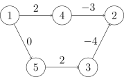
The shortest path from \(1 \to 2\) is \(1 \to 5 \to 3 \to 2\), length \(−2\).

But what if we add \(5\) to every edge weight?

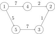
The shortest path from \(1 \to 2\) on the new graph becomes \(1 \to 4 \to 2\), which is no longer the actual shortest path.

The Johnson algorithm uses another method to reweight edges.

We create a virtual vertex (let its index be \(0\)). Connect this vertex to all other vertices with edges of weight \(0\).

Next, run the Bellman–Ford algorithm to find the shortest path from vertex \(0\) to all other vertices, denoted \(h_i\).

If there is an edge from \(u\) to \(v\) with weight \(w\), we reset the edge weight to \(w+h_u-h_v\).

Then, starting from each vertex as source, run Dijkstra \(n\) times to find the shortest path between any two vertices.

The initial Bellman–Ford algorithm is not a bottleneck in time. If Dijkstra is implemented with priority_queue, the algorithm's time complexity is \(O(nm\log m)\).

Correctness Proof

Why is this edge reweighting method correct?

Before discussing this, let's discuss a physics concept—potential energy.

Potential energies like gravitational potential energy and electric potential energy have a characteristic: the change in potential energy depends only on the relative positions of the start and end points, not on the path taken.

Another characteristic: the absolute value of potential energy often depends on where the zero potential point is set, but no matter where it is set, the difference in potential energy between two points is constant.

Now back to the topic.

On the reweighted graph, the length of a path \(s \to p_1 \to p_2 \to \dots \to p_k \to t\) from \(s\) to \(t\) is expressed as:

\((w(s,p_1)+h_s-h_{p_1})+(w(p_1,p_2)+h_{p_1}-h_{p_2})+ \dots +(w(p_k,t)+h_{p_k}-h_t)\)

Simplifying:

\(w(s,p_1)+w(p_1,p_2)+ \dots +w(p_k,t)+h_s-h_t\)

No matter which path we take from \(s\) to \(t\), the value \(h_s-h_t\) is constant, which matches the property of potential energy!

For convenience, we call \(h_i\) the potential of vertex \(i\).

The length expression of the shortest path from \(s \to t\) on the new graph consists of two parts: the sum of edge weights is the shortest path from \(s \to t\) on the original graph, and the latter is the potential difference between the two points. Since the potential difference between two points is constant, the shortest path from \(s \to t\) on the original graph corresponds to the shortest path from \(s \to t\) on the new graph.

Here we have solved half of the correctness proof—we have proved that the shortest path on the reweighted graph is still the original shortest path. Next we need to prove that all edge weights on the new graph are non-negative, because on non-negative weighted graphs, Dijkstra's algorithm can guarantee correct results.

According to the triangle inequality, any edge \((u,v)\) satisfies: \(h_v \leq h_u + w(u,v)\). The reweighted edge weight is \(w'(u,v)=w(u,v)+h_u-h_v \geq 0\). This proves that all edge weights on the new graph are non-negative.

Thus, we have proved the correctness of Johnson's algorithm.

Comparison of Methods

Shortest Path Algorithm	Floyd	Bellman–Ford	Dijkstra	Johnson
Shortest Path Type	All-Pairs	Single-Source	Single-Source	All-Pairs
Applicable Graph	Any Graph	Any Graph	Non-negative	Any Graph
Can Detect Negative Cycle?	Yes	Yes	No	Yes
Time Complexity	\(O(N^3)\)	\(O(NM)\)	\(O(M\log M)\)	\(O(NM\log M)\)

Note: The Dijkstra algorithm in the table uses priority_queue for complexity calculation.

Outputting the Path

Maintain a pre array, record how the next vertex is transferred when updating distances, and recursively output the path before the algorithm ends.

For example, Floyd records pre[i][j] = k;, while Bellman–Ford and Dijkstra generally record pre[v] = u.

Some Special Cases

• Shortest path on graphs with edge weights only \(0\) and \(1\): 0-1 BFS;
• Shortest path problems allowing at most \(k\) operations to change path cost, etc.: Layered Graph Shortest Path.

References and Notes

---

1. Introduction to Algorithms (3^rd Edition Chinese Translation), Mechanical Industry Press, 2013, pp. 384–385. ↩

---

本页面最近更新：，更新历史
发现错误？想一起完善？ 在 GitHub 上编辑此页！
本页面贡献者：OI-wiki
本页面的全部内容在 CC BY-SA 4.0 和 SATA 协议之条款下提供，附加条款亦可能应用