Minimum Spanning Tree
Definition
Before reading the following content, please be sure to read the Graph Theory Related Concepts and Tree Basics sections, and understand the following definitions:
- Spanning subgraph
- Spanning tree
We define the Minimum Spanning Tree (MST) of an undirected connected graph as the spanning tree with the minimum sum of edge weights.
Note: Only connected graphs have spanning trees, while for disconnected graphs, only spanning forests exist.
Kruskal's Algorithm
Kruskal's algorithm is a common and easy-to-write minimum spanning tree algorithm, invented by Kruskal. The basic idea of the algorithm is to add edges from smallest to largest, making it a greedy algorithm.
Prerequisites
Disjoint Set Union (DSU), Greedy, Graph Storage.
Implementation
Illustration:
Pseudocode:
Although the algorithm is simple, it requires appropriate data structures to support it... Specifically, maintain a forest, query whether two nodes are in the same tree, and connect two trees.
More abstractly, maintain a collection of sets, query whether two elements belong to the same set, and merge two sets.
Among these, querying whether two points are connected and connecting two points can be maintained using a disjoint set union.
If an \(O(m\log m)\) sorting algorithm is used, along with an \(O(m\alpha(m, n))\) or \(O(m\log n)\) disjoint set union, a Kruskal's algorithm with time complexity \(O(m\log m)\) can be obtained.
Proof
The idea is simple: to construct a minimum spanning tree, we start from the edge with the smallest weight and add edges in increasing order of weight. If adding an edge creates a cycle, discard that edge. Continue until \(n-1\) edges are added, forming a tree.
Proof: Use induction to prove that at any time, the edge set selected by Kruskal's algorithm is contained in some MST.
Base case: At the start of the algorithm, it obviously holds (a minimum spanning tree exists).
Inductive step: Assume it holds at some moment, with the current edge set \(F\). Let \(T\) be this MST, and consider the next edge \(e\) to be added.
If \(e\) belongs to \(T\), then it holds.
Otherwise, \(T+e\) must contain a cycle. Consider another edge \(f\) on this cycle that does not belong to \(F\) (at least one exists).
First, the weight of \(f\) cannot be less than that of \(e\); otherwise, \(f\) would have been selected before \(e\).
Second, the weight of \(f\) cannot be greater than that of \(e\); otherwise, \(T+e-f\) would be a spanning tree better than \(T\).
Thus, \(T+e-f\) contains \(F\) and is also a minimum spanning tree, completing the induction.
Example
Luogu P1195 Pocket Sky
There are \(n\) clouds, and you need to connect them into \(k\) cotton candies. Connecting cloud \(X_i\) and \(Y_i\) requires a cost of \(L_i\). Find the minimum total cost.
Example Code
1 2 3 4 5 6 7 8 9 10 11 12 13 14 15 16 17 18 19 20 21 22 23 24 25 26 27 28 29 30 31 32 33 34 35 36 37 38 39 40 41 42 43 44 45 46 47 48 49 50 51 52 53 54 55 56 57 58 59 60 61 62 63 64 65 66 67 68 69 | |
1 2 3 4 5 6 7 8 9 10 11 12 13 14 15 16 17 18 19 20 21 22 23 24 25 26 27 28 29 30 31 32 33 34 35 36 37 38 39 40 41 42 43 44 45 46 47 48 49 50 51 52 53 54 55 56 57 58 | |
1 2 3 4 5 6 7 8 9 10 11 12 13 14 15 16 17 18 19 20 21 22 23 24 25 26 27 28 29 30 31 32 33 34 35 36 37 38 39 40 41 42 43 44 45 46 47 48 49 50 51 52 53 54 55 56 57 58 59 60 61 62 63 64 65 66 67 68 69 70 71 72 73 74 75 76 77 78 79 80 81 82 83 84 85 86 87 88 89 90 91 92 | |
Prim's Algorithm
Prim's algorithm is another common and easy-to-write minimum spanning tree algorithm. The basic idea is to start from a single node and continuously add nodes (as opposed to Kruskal's algorithm which adds edges).
Implementation
Illustration:
Specifically, each time we select the node with the smallest distance and update the distances of other nodes with the new edge.
This is similar to Dijkstra's algorithm: each time we find the node with the smallest distance, either by brute force or using a heap.
Heap optimization is similar to Dijkstra's heap optimization. However, if using a binary heap or other heaps that do not support \(O(1)\) decrease-key, the complexity is not better than Kruskal's, and the constant factor is larger. Therefore, Kruskal's algorithm is generally used. On dense graphs, especially complete graphs, the brute-force Prim's complexity is better than Kruskal's, but it may not actually run faster.
Brute force: \(O(n^2+m)\).
Binary heap: \(O((n+m) \log n)\).
Fibonacci heap: \(O(n \log n + m)\).
Pseudocode:
Note: The above code only computes the weight of the minimum spanning tree. To output the actual tree, you need to record which edge each node's \(dis\) represents.
Code Implementation
1 2 3 4 5 6 7 8 9 10 11 12 13 14 15 16 17 18 19 20 21 22 23 24 25 26 27 28 29 30 31 32 33 34 35 36 37 38 39 40 41 42 43 44 45 46 47 48 49 50 51 52 53 54 55 56 57 58 59 60 | |
Proof
Start from any node, dividing nodes into two categories: added and not added.
Each time, among the unadded nodes, find the node with the minimum edge weight to any added node.
Then add this node and connect it with that minimum-weight edge.
Repeat \(n-1\) times.
Proof: Again, we show that at each step, there exists a minimum spanning tree containing the current edge set.
Base case: With only one node, it obviously holds.
Inductive step: If it holds at some step, with current edge set \(F\) belonging to MST \(T\), and we are about to add edge \(e\).
If \(e\) belongs to \(T\), then it holds.
Otherwise, consider another edge \(f\) on the cycle in \(T+e\) that can be added to the current edge set.
First, the weight of \(f\) cannot be less than that of \(e\); otherwise, \(f\) would have been chosen instead of \(e\).
Second, the weight of \(f\) cannot be greater than that of \(e\); otherwise, \(T+e-f\) would be a smaller spanning tree.
Thus, \(e\) and \(f\) have equal weights, and \(T+e-f\) is also a minimum spanning tree containing \(F\).
Borůvka's Algorithm
Next, we introduce another algorithm for solving the minimum spanning tree problem—Borůvka's algorithm. This algorithm combines ideas from the previous two algorithms. It can be used to find the minimum spanning forest of an undirected graph (for a connected undirected graph, it is the minimum spanning tree).
Borůvka's algorithm has advantages in problems where edges have special properties. For example, the complete graph problem in CF888G.
To describe the algorithm, we need some definitions:
- Define \(E'\) as the edges of the current minimum spanning forest. During the algorithm, we gradually add edges to \(E'\). Define a connected component as a vertex set \(V'\subseteq V\) such that any two vertices \(u\), \(v\) in this set are connected (mutually reachable) in the subgraph formed by the edges in \(E'\).
- Define the minimum edge of a connected component as the edge with the smallest weight connecting it to another component.
Initially, \(E'=\varnothing\), and each vertex is its own connected component:
- Compute which connected component each vertex belongs to. Set each component to have "no minimum edge".
- Traverse each edge \((u, v)\). If \(u\) and \(v\) are in different components, use this edge's weight to update the minimum edge of the components containing \(u\) and \(v\).
- If all components have no minimum edge, exit. At this point, \(E'\) is the edge set of the minimum spanning forest. Otherwise, add the minimum edge of each component that has one to \(E'\), and return to step 1.
The following animation illustrates an example (image from Wikipedia):
When the original graph is connected, the number of components at least halves each iteration, so the algorithm iterates at most \(O(\log V)\) times. For disconnected graphs, it is equivalent to multiple subproblems. Thus, the algorithm complexity is \(O(E\log V)\). Pseudocode (modified from Wikipedia):
Note: Edge comparisons often require a secondary key (e.g., sorting by edge ID) to break ties when edge weights are equal.
Exercises
Uniqueness of Minimum Spanning Tree
Consider the uniqueness of the minimum spanning tree. If an edge is not in the edge set of the minimum spanning tree and can replace another edge with the same weight that is in the edge set of the minimum spanning tree, then the minimum spanning tree is not unique.
For Kruskal's algorithm, we can compute how many edges of the current weight can be added and how many are actually added. If these two numbers differ, it means these edges form a cycle with previous edges (this cycle contains at least two edges of the current weight; otherwise, based on the disjoint set union, this edge could not be added), indicating the minimum spanning tree is not unique.
To find edges with the same weight as the current edge, we only need to record head and tail pointers and use a monotonic queue to solve this problem efficiently in \(O(\alpha(m))\) time (where \(m\) is the number of edges), essentially the same as the original algorithm.
Example: POJ 1679
1 2 3 4 5 6 7 8 9 10 11 12 13 14 15 16 17 18 19 20 21 22 23 24 25 26 27 28 29 30 31 32 33 34 35 36 37 38 39 40 41 42 43 44 45 46 47 48 49 50 51 52 53 54 55 56 57 58 59 60 61 62 | |
Second Minimum Spanning Tree
Non-strict Second Minimum Spanning Tree
Definition
In an undirected graph, the spanning tree with the smallest sum of edge weights that is greater than or equal to the sum of the minimum spanning tree's edge weights.
Solution Method
- Find the minimum spanning tree \(T\) of the undirected graph, and let its weight sum be \(M\).
- For each unselected edge \(e = (u,v,w)\), find the edge with the maximum weight \(e' = (s,t,w')\) on the path from \(u\) to \(v\) in \(T\). Then replace \(e'\) with \(e\) in \(T\) to obtain a spanning tree \(T'\) with weight sum \(M' = M + w - w'\).
- Take the minimum among all such \(M'\).
How to find the maximum edge weight on the path between \(u\) and \(v\)?
We can use binary lifting to maintain this. Preprocess each node's \(2^i\)-th ancestor and the maximum edge weight on the path to that ancestor. Then, during binary lifting for LCA, we can directly obtain the maximum edge weight.
Strict Second Minimum Spanning Tree
Definition
In an undirected graph, the spanning tree with the smallest sum of edge weights that is strictly greater than the sum of the minimum spanning tree's edge weights.
Solution Method
Consider the solution process for the non-strict second minimum spanning tree. Why is the obtained solution non-strict?
Because the minimum spanning tree ensures that the maximum edge weight on the path between \(u\) and \(v\) in the tree is no greater than the maximum edge weight on any other path from \(u\) to \(v\). In other words, when the weight of the edge used for replacement equals the weight of the replaced edge in the original spanning tree, the resulting second minimum spanning tree is non-strict.
The solution is natural: while maintaining the maximum edge weight on the path to the \(2^i\)-th ancestor, also maintain the strict second maximum edge weight. When the weight of the replacement edge equals the maximum edge weight on the path in the original tree, use the strict second maximum value for replacement.
This process can be solved using binary lifting with complexity \(O(m \log m)\).
Code Implementation
1 2 3 4 5 6 7 8 9 10 11 12 13 14 15 16 17 18 19 20 21 22 23 24 25 26 27 28 29 30 31 32 33 34 35 36 37 38 39 40 41 42 43 44 45 46 47 48 49 50 51 52 53 54 55 56 57 58 59 60 61 62 63 64 65 66 67 68 69 70 71 72 73 74 75 76 77 78 79 80 81 82 83 84 85 86 87 88 89 90 91 92 93 94 95 96 97 98 99 100 101 102 103 104 105 106 107 108 109 110 111 112 113 114 115 116 117 118 119 120 121 122 123 124 125 126 127 128 129 130 131 132 133 134 135 136 137 138 139 140 141 142 143 144 145 146 147 148 149 150 151 152 153 154 | |
Bottleneck Spanning Tree
Definition
A bottleneck spanning tree of an undirected graph \(G\) is a spanning tree whose maximum edge weight is the smallest among all spanning trees of \(G\).
Properties
A minimum spanning tree is a bottleneck spanning tree, but the converse is not necessarily true. That is, a minimum spanning tree is always a bottleneck spanning tree, but a bottleneck spanning tree may not be a minimum spanning tree.
To prove that a minimum spanning tree is always a bottleneck spanning tree, we can use contradiction: Let the maximum edge weight in the minimum spanning tree be \(w\). If the minimum spanning tree is not a bottleneck spanning tree, then all edge weights in the bottleneck spanning tree are less than \(w\). Remove the longest edge from the original minimum spanning tree and connect the two resulting trees with an edge from the bottleneck spanning tree. The new spanning tree will have a smaller total weight than the original minimum spanning tree, leading to a contradiction.
Example
POJ 2395 Out of Hay
Given n farms and m edges, farms numbered 1 to n, a person needs to travel from farm 1 to other farms. Find the maximum amount of water he needs to carry during the journey. Note that he can replenish water at each farm, and the total path length should be minimized. The problem asks for the maximum edge weight in the bottleneck tree, which can be solved by finding the minimum spanning tree.
Minimum Bottleneck Path
Definition
A minimum bottleneck path from x to y in an undirected graph \(G\) is a simple path such that the maximum edge weight on this path is the smallest among all simple paths from x to y.
Properties
By the definition of the minimum spanning tree, the maximum edge weight on the minimum bottleneck path from x to y equals the maximum edge weight on the path from x to y in the minimum spanning tree. Although the minimum spanning tree is not unique, the maximum edge weight on the path from x to y is the same for all minimum spanning trees and is the minimum possible. That is, the path from x to y in any minimum spanning tree is a minimum bottleneck path.
However, not all minimum bottleneck paths exist as a simple path from x to y in some minimum spanning tree.
For example, consider the following graph:
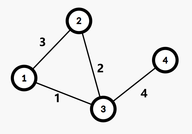
The minimum bottleneck paths from 1 to 4 are clearly: 1-2-3-4 and 1-3-4.
But 1-2 does not appear in any minimum spanning tree.
Applications
Since minimum bottleneck paths are not unique, we typically ask for the maximum edge weight on a minimum bottleneck path.
That is, we need to find the max on a chain in the minimum spanning tree.
Binary lifting or heavy-light decomposition can solve this; we will not elaborate here.
Kruskal Reconstruction Tree
Definition
While running Kruskal's algorithm, we add edges in increasing order. We follow this order.
First, create \(n\) sets, each containing exactly one node with weight \(0\).
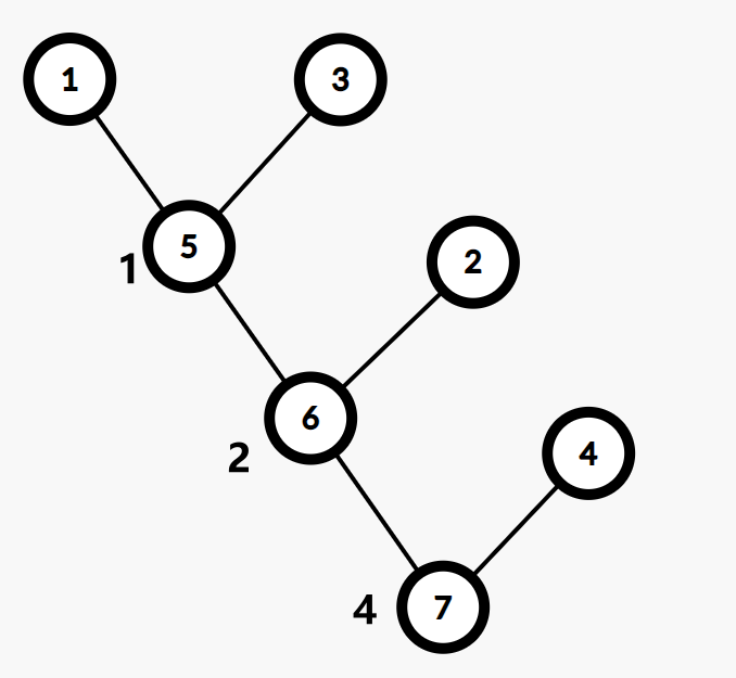
Each time we add an edge merging two sets, we create a new node with weight equal to the added edge's weight. Set the roots of the two sets as the left and right children of this new node. Then merge the two sets and the new node into one set, with the new node as the root.
After \(n-1\) rounds, we obtain a binary tree with exactly \(n\) leaves, and each non-leaf node has exactly two children. This tree is called the Kruskal reconstruction tree.
For example:
The Kruskal reconstruction tree for this graph is:
Properties
It is not hard to see that the minimum of the maximum edge weights over all simple paths between two points in the original graph = the maximum edge weight on the simple path between the two points in the minimum spanning tree = the weight of the LCA of the two points in the Kruskal reconstruction tree.
That is, all points \(y\) such that the minimum of the maximum edge weights on simple paths to \(x\) is \(\leq val\) are exactly the leaves of a certain subtree in the Kruskal reconstruction tree, and that subtree contains all such points.
We find the shallowest node on the path from \(x\) to the root in the Kruskal reconstruction tree with weight \(\leq val\). This is precisely the root of the subtree containing all such points.
If we need the maximum of the minimum edge weights over all simple paths between two points in the original graph, run Kruskal's algorithm adding edges in decreasing order of weight.
「LOJ 137」Minimum Bottleneck Path (Enhanced)
1 2 3 4 5 6 7 8 9 10 11 12 13 14 15 16 17 18 19 20 21 22 23 24 25 26 27 28 29 30 31 32 33 34 35 36 37 38 39 40 41 42 43 44 45 46 47 48 49 50 51 52 53 54 55 56 57 58 59 60 61 62 63 64 65 66 67 68 69 70 71 72 73 74 75 76 77 78 79 80 81 82 83 84 85 86 87 88 89 90 91 92 93 94 95 96 97 98 99 100 101 102 103 104 105 106 107 108 109 110 111 112 113 114 115 116 117 118 119 120 121 122 123 124 125 126 127 128 129 130 131 132 133 134 135 136 137 138 | |
NOI 2018 Return
First, precompute the shortest path from each node to the root.
Construct the maximum spanning tree based on altitude. Clearly, the nodes reachable in each query are those on the path from the query point in the maximum spanning tree with minimum edge weight \(> p\).
By the properties of the Kruskal reconstruction tree, these nodes are all in a single subtree and are exactly its leaves.
That is, we only need to compute the minimum weight among leaves in each subtree of the Kruskal reconstruction tree to support subtree queries.
The root node for the query can be found using binary lifting on the Kruskal reconstruction tree.
Time complexity: \(O((n+m+Q) \log n)\).
本页面最近更新:,更新历史
发现错误?想一起完善? 在 GitHub 上编辑此页!
本页面贡献者:OI-wiki
本页面的全部内容在 CC BY-SA 4.0 和 SATA 协议之条款下提供,附加条款亦可能应用