Block Forest
Before reading the following content, please make sure to understand the Graph Theory Concepts section.
Related reading: Cut Vertices and Bridges.
Introduction
It is well known that trees (or forests) have nice properties and are easy to maintain with many common data structures.
General graphs do not have such good properties, but fortunately, sometimes we can transform certain problems on general graphs into problems on trees.
The Block Forest or Round-square tree1 is a method to convert a graph into a tree. This article will introduce the construction, properties, and some applications of the block forest.
Due to space limitations, some conclusions in this article are not proven; readers can understand or prove them on their own.
Definition
The block forest was originally a tool for handling cactus graphs (undirected graphs where each edge belongs to at most one simple cycle). However, by exploring more of its properties, we can sometimes use it on general undirected graphs.
To introduce the block forest, we must first introduce biconnected components.
A biconnected graph can be defined as: for any two distinct vertices in the graph, there are at least two vertex-disjoint paths between them.
Vertex-disjoint means the paths do not share any vertices (simple paths), and the intersection of the two paths is empty (of course, the paths necessarily pass through the starting and ending points, which are not considered here).
It can be noticed that it is difficult to define whether a graph with only one vertex is biconnected. For now, we do not consider graphs with a single vertex.
An almost equivalent definition is: a graph with no cut vertices.
This definition fails only when the graph has exactly two vertices and one edge connecting them. It has no cut vertex, but we cannot find two disjoint paths because there is only one path.
(Alternatively, we can think of that single path being counted twice; indeed, they do not intersect because they do not pass through other vertices.)
Although the original definition is indeed the former, for convenience, we adopt the latter as the definition of a biconnected graph.
The biconnected components of a graph are its maximal biconnected subgraphs.
Unlike strongly connected components, a vertex may belong to multiple biconnected components, but an edge belongs to exactly one biconnected component (if we adopt the former definition, an edge might not belong to any biconnected component).
In the block forest, each original vertex corresponds to a round vertex, and each biconnected component corresponds to a square vertex.
Thus, there are \(n+c\) vertices in total, where \(n\) is the number of vertices in the original graph, and \(c\) is the number of biconnected components in the original graph.
For each biconnected component, its corresponding square vertex connects to every vertex in that biconnected component.
Each biconnected component forms a "star graph", and multiple "star graphs" are connected via the cut vertices of the original graph (since the separating vertices of biconnected components are cut vertices).
Clearly, each edge in the block forest connects a round vertex and a square vertex.
The following figures show the biconnected components of a graph and the corresponding block forest structure.2
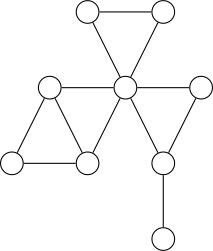
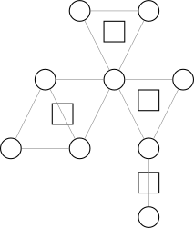
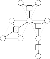
The number of vertices in the block forest is less than \(2n\), because the number of cut vertices is less than \(n\). Therefore, please note that various array sizes should be doubled.
In fact, if the original graph is connected, the "block forest" is a tree. If the original graph has \(k\) connected components, its block forest will form a forest of \(k\) trees.
If a connected component in the original graph has only one vertex, it needs to be analyzed case by case. We do not consider isolated vertices in the following discussion.
Process
For a given graph, how do we construct its block forest? First, note that if the graph is not connected, we can split it into each connected component and consider them separately. Thus, we only consider connected graphs.
Since the block forest is based on biconnected components, and biconnected components are based on cut vertices, we only need to use an algorithm similar to finding cut vertices.
The common algorithm for finding cut vertices is Tarjan's algorithm. If you understand it, the following content will be straightforward. If not, it's okay.
We skip Tarjan's algorithm for cut vertices and directly introduce the algorithm used for the block forest (which is actually a variant of Tarjan's):
Perform DFS on the graph, using two key arrays dfn and low (similar to Tarjan).
dfn[u] stores the DFS order of vertex \(u\), i.e., the order in which \(u\) is first visited.
low[u] stores the smallest DFS order among vertices reachable from any vertex \(v\) in the DFS subtree of \(u\) via at most one back edge or a tree edge to the parent.
If you haven't heard of Tarjan's algorithm, this might be hard to understand. Let's look at an example:
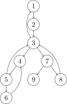
(Note that this graph is essentially equivalent to the one in the image above.)
Here, tree edges are drawn as straight lines from top to bottom, and back edges are drawn as curved lines from bottom to top. The numbers next to the vertices are their DFS orders.
The low array is as follows:
| \(i\) | \(1\) | \(2\) | \(3\) | \(4\) | \(5\) | \(6\) | \(7\) | \(8\) | \(9\) |
|---|---|---|---|---|---|---|---|---|---|
| \(\mathrm{low}[i]\) | \(1\) | \(1\) | \(1\) | \(3\) | \(3\) | \(4\) | \(3\) | \(3\) | \(7\) |
It's not too hard to understand. Note that the low value for \(9\) is \(7\), which differs from some cut-finding implementations because, for convenience, we allow moving upward via the parent edge. However, the main idea is the same.
We can easily write a DFS function to compute dfn and low (initialize the dfn array to zero):
Implementation
1 2 3 4 5 6 7 8 9 10 | |
1 2 3 4 5 6 7 8 9 | |
Next, we consider the relationship between biconnected components, the DFS tree, and these two arrays.
We can observe that each biconnected component corresponds to a connected subtree in the DFS tree and contains at least two vertices; in particular, the topmost vertex connects downward to only one vertex.
We also notice that each tree edge belongs to exactly one biconnected component.
Consider the topmost vertex \(u\) of a biconnected component in the DFS tree. We determine this biconnected component at \(u\) because the subtree of \(u\) contains all information about the component.
Since there are at least two vertices, consider the next vertex \(v\) in this biconnected component. There is a tree edge between \(u\) and \(v\).
It is not hard to see that \(\mathrm{low}[v]=\mathrm{dfn}[u]\) must hold.
More precisely, for a tree edge \(u\to v\), \(u\) and \(v\) are in the same biconnected component, and \(u\) is the shallowest vertex in that component if and only if \(\mathrm{low}[v]=\mathrm{dfn}[u]\).
Thus, during DFS, we can identify where biconnected components exist, but we cannot yet precisely determine the set of vertices in a biconnected component.
This is not difficult to handle. We can maintain a stack during DFS to store vertices whose biconnected component membership (there may be multiple) has not been determined.
When we find a biconnected component, all vertices in the component except \(u\) are concentrated at the top of the stack. We simply pop from the stack until \(v\) is popped.
Of course, we can process the popped vertices simultaneously by connecting them to the newly created square vertex. Finally, we also connect \(u\) to the square vertex.
This naturally completes the construction of the block forest. We can label square vertices starting from \(n+1\), which effectively distinguishes round vertices from square vertices.
This part may not be explained clearly enough. Below is a code snippet with detailed comments, helpful output statements, and a sample test case. It is recommended that readers copy the code and practice understanding it, as code is the best way to grasp the concept (do not forget to enable c++11).
Implementation
1 2 3 4 5 6 7 8 9 10 11 12 13 14 15 16 17 18 19 20 21 22 23 24 25 26 27 28 29 30 31 32 33 34 35 36 37 38 39 40 41 42 43 44 45 46 47 48 49 50 51 52 53 54 55 56 57 58 59 | |
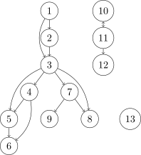
Here is a test case:
1 2 3 4 5 6 7 8 9 10 11 12 13 14 15 16 | |
The graph corresponding to this example (including multiple edges and isolated vertices):
Examples
We discuss some example problems that can be solved using the block forest.
「APIO2018」Iron Man Triathlon
Brief Description
Given a simple undirected graph, count the number of triples \(\langle s, c, f \rangle\) (with \(s, c, f\) distinct) such that there exists a simple path from \(s\) through \(c\) to \(f\).
Solution
When talking about simple paths, we must mention a nice property about biconnected components: for any two vertices in a biconnected component, the union of all simple paths between them exactly equals the biconnected component.
That is, for any two distinct vertices \(u,v\) in the same biconnected component, there always exists a simple path from \(u\) to \(v\) passing through any given third vertex \(w\) in the same biconnected component.
Proof of this property:
- Obviously, if a simple path leaves the biconnected component, it cannot return to it; otherwise, it would contradict the definition of a biconnected component.
- Thus, we only need to prove that in a biconnected graph with three distinct vertices \(u,v,c\), there exists a simple path from \(u\) to \(v\) passing through \(c\).
- First, exclude the case of exactly two vertices; it satisfies the property but cannot have three distinct vertices.
- For the remaining cases, consider constructing a network flow model: connect the source to \(c\) with capacity \(2\), and connect \(u\) and \(v\) to the sink with capacity \(1\).
- For each undirected edge \(\langle x,y\rangle\) in the original graph, create a directed edge from \(x\) to \(y\) with capacity \(1\), and another from \(y\) to \(x\) with capacity \(1\).
- Finally, assign a capacity of \(1\) to every vertex except the source, sink, and \(c\), which can be achieved by vertex splitting.
- Since the edge from the source to \(c\) has capacity \(2\), if the maximum flow of this network is \(2\), then there must be a path through \(c\).
- By the max-flow min-cut theorem, obviously the minimum cut is at most \(2\). Next, we prove the minimum cut is greater than \(1\).
- This is equivalent to proving that cutting any single edge of capacity \(1\) cannot disconnect the source and sink.
- Consider cutting the edge connecting \(u\) or \(v\) to the sink. By the first definition of biconnected components, there must exist a simple path from \(c\) to the other uncut vertex.
- Consider cutting an edge formed by splitting a vertex (i.e., deleting a vertex). By the second definition of biconnected components, the remaining graph is still connected.
- Consider cutting an edge corresponding to an original edge (i.e., deleting an edge). This is weaker than deleting a vertex, so a path obviously exists.
- Thus, we have proved the minimum cut is greater than \(1\), so the maximum flow equals \(2\). QED.
What does this conclusion tell us? It tells us: consider the path between two round vertices in the block forest. The set of round vertices adjacent to the square vertices along this path equals the set of vertices on any simple path between the two original vertices.
Returning to the problem, fix \(s\) and \(f\), and count the number of valid \(c\). Clearly, the number of valid \(c\) equals the size of the union of all simple paths between \(s\) and \(f\), minus \(2\) (removing \(s\) and \(f\) themselves).
After constructing the block forest for the original graph, the number of vertices on any simple path between two vertices relates to the number of square vertices (biconnected components) and round vertices along their path in the block forest.
Next is a common technique for block forests: assign appropriate weights to vertices when performing path statistics.
In this problem, each square vertex is assigned a weight equal to the size of its corresponding biconnected component, and each round vertex is assigned a weight of \(-1\).
With this weighting, the sum of vertex weights along the path between two round vertices in the block forest exactly equals the size of the union of simple paths in the original graph minus \(2\).
The problem reduces to computing the sum of path weights between all pairs of round vertices in the block forest.
Alternatively, consider counting each vertex's contribution to the answer: its weight multiplied by the number of paths passing through it. This can be computed via simple tree DP.
Finally, do not forget to handle disconnected graphs. Below is the corresponding code:
Reference Code
1 2 3 4 5 6 7 8 9 10 11 12 13 14 15 16 17 18 19 20 21 22 23 24 25 26 27 28 29 30 31 32 33 34 35 36 37 38 39 40 41 42 43 44 45 46 47 48 49 50 51 52 53 54 55 56 57 58 59 60 61 62 63 64 65 66 67 68 69 70 71 72 73 74 75 76 77 | |
By the way, the answer for the test case above in this problem is \(212\).
Codeforces #487 E. Tourists
Brief Description
Given a simple connected undirected graph, support two types of operations:
-
Modify the weight of a vertex.
-
Query the minimum weight among all vertices on any simple path between two given vertices.
Solution
Similarly, we construct the block forest of the original graph. Let the weight of each square vertex be the minimum weight among its adjacent round vertices. The problem reduces to querying the minimum weight on a path.
Path minimum can be maintained using heavy-light decomposition and segment trees. But what about modifications?
Modifying the weight of a round vertex requires updating all adjacent square vertices, which could easily degrade to \(O(n)\) modifications.
Here, we utilize the fact that the block forest is a tree: let the weight of a square vertex be the minimum weight among its child round vertices. Then, when modifying a round vertex, we only need to update its parent square vertex.
For maintaining square vertices, simply use a multiset for each square vertex to store the set of weights.
Note that when querying, if the LCA is a square vertex, we also need to consider the weight of its parent round vertex.
Note: The number of vertices in the block forest should be doubled compared to the original graph to avoid array out-of-bounds.
Reference Code
1 2 3 4 5 6 7 8 9 10 11 12 13 14 15 16 17 18 19 20 21 22 23 24 25 26 27 28 29 30 31 32 33 34 35 36 37 38 39 40 41 42 43 44 45 46 47 48 49 50 51 52 53 54 55 56 57 58 59 60 61 62 63 64 65 66 67 68 69 70 71 72 73 74 75 76 77 78 79 80 81 82 83 84 85 86 87 88 89 90 91 92 93 94 95 96 97 98 99 100 101 102 103 104 105 106 107 108 109 110 111 112 113 114 115 116 117 118 119 120 121 122 123 124 125 126 127 128 129 130 131 132 133 134 135 136 137 138 139 140 141 142 143 144 145 | |
「SDOI2018」Strategy Game
Brief Description
Given a simple connected undirected graph. There are \(q\) queries:
Each query gives a vertex set \(S\) (\(2 \le |S| \le n\)). Ask how many vertices \(u\) satisfy \(u \notin S\) and after removing \(u\), the vertices in \(S\) are not all in the same connected component.
Each test case contains multiple groups of data.
Solution
First, construct the block forest. The problem reduces to counting the number of round vertices in the connected subgraph of the block forest corresponding to \(S\), minus \(|S|\).
How to count the number of round vertices in a connected subgraph? One method:
Assign the weight of each round vertex to the edge between it and its parent square vertex. The problem becomes summing edge weights, which can be solved similarly to one solution for 「SDOI2015」Treasure Hunt.
That is, sort the vertices in \(S\) by DFS order, compute the sum of distances between consecutive vertices in sorted order (including the distance between the first and last), and the answer is half of this sum because each edge is traversed twice.
Finally, if the shallowest vertex in the subgraph is a round vertex, add \(1\) to the answer because we did not count it.
Since there are multiple groups of data, remember to initialize arrays.
Reference Code
1 2 3 4 5 6 7 8 9 10 11 12 13 14 15 16 17 18 19 20 21 22 23 24 25 26 27 28 29 30 31 32 33 34 35 36 37 38 39 40 41 42 43 44 45 46 47 48 49 50 51 52 53 54 55 56 57 58 59 60 61 62 63 64 65 66 67 68 69 70 71 72 73 74 75 76 77 78 79 80 81 82 83 84 85 86 87 88 89 90 91 92 93 94 | |
Exercises
External Links
immortalCO, Block Forest — A Powerful Tool for Handling Cactus Graphs, Universal OJ.
References and Notes
-
In 2017, Chen Junkun defined and named the block forest structure in his IOI2017 Chinese National Team paper "《神奇的子图》命题报告及其拓展" ("The Magical Subgraph" Problem Report and Extensions). ↩
-
Chen Junkun, "平凡的圆方树和神奇的(
动态)动态规划" ("The Ordinary Block Forest and the Magical (Dynamic) Dynamic Programming"), NOI2018 Winter Camp, page 4. ↩
本页面最近更新:,更新历史
发现错误?想一起完善? 在 GitHub 上编辑此页!
本页面贡献者:OI-wiki
本页面的全部内容在 CC BY-SA 4.0 和 SATA 协议之条款下提供,附加条款亦可能应用