Stoer–Wagner Algorithm
Definition
Since the concept of source and sink is removed, we need to redefine the concept of a cut.
(Actually, the definition of a cut in the network flow section does not match Wikipedia, but since the cuts we usually encounter are in the context of "minimum cut problems with source and sink," this concept has become conventional.)
Cut
A set of edges whose removal disconnects a network flow graph (i.e., splits it into two subgraphs) is called a cut of the graph.
That is: In an undirected graph \(G = (V, E)\), let \(C\) be a set of arcs in \(G\). If removing all arcs in \(C\) from \(G\) makes \(G\) disconnected, then \(C\) is called a cut of graph \(G\).
Minimum Cut Problem with Source and Sink
Same as the definition in Minimum Cut.
Minimum Cut Problem without Source and Sink
The cut with the smallest sum of arc weights. Also known as the global minimum cut.
Clearly, directly running network flow algorithms is not feasible in terms of complexity.
Stoer–Wagner Algorithm
Introduction
The Stoer–Wagner algorithm was proposed in 1995 by Mechthild Stoer and Frank Wagner. It is an algorithm that solves the global minimum cut problem on undirected positive-weighted graphs through a recursive approach.
Properties
The algorithm complexity is \(O(|V||E| + |V|^{2}\log|V|)\), which can generally be approximated as \(O(|V|^3)\).
Its implementation is based on the following fundamental fact: Let \(S, T\) be any two vertices in graph \(G\). Then for any cut \(C\) of graph \(G\), either \(S\) and \(T\) are in the same connected component, or \(C\) is an \({S-T}\) cut.
Procedure
- Arbitrarily select two vertices \(s, t\) in graph \(G\), and compute the \(S-T\) minimum cut of graph \(G\) (defined as the cut of phase) using these two as source and sink, updating the current answer.
- "Merge" vertices \(s\) and \(t\). If \(|V|\) in graph \(G\) is greater than \(1\), return to step 1.
- Output the minimum value among all cut of phase.
Merging vertices \(s\) and \(t\): Remove the edge \((s, t)\) between \(s\) and \(t\). For any vertex \(k\) in \(G \setminus \{s, t\}\), remove \((t, k)\) and add its edge weight \(d(t, k)\) to \(d(s, k)\).
Explanation: If \(s\) and \(t\) are in the same connected component, for a vertex \(k\) in \(G \setminus \{s, t\}\), if \((k, s) \in C_{\min}\), then \((k, t) \in C_{\min}\) must also hold. Otherwise, because \(s\) and \(t\) are connected, and \(k\) and \(t\) are connected, \(s\) and \(k\) would be in the same connected component. In this case, \(C = C_{\min} \setminus \{(t, k)\}\) would be better than \(C_{\min}\). The converse is also true. Therefore, \(s\) and \(t\) can be treated as the same vertex.
Step 1 considers the case where \(s\) and \(t\) are not in the same connected component, while step 2 considers the remaining cases. Since each execution of step 2 reduces \(|V|\) by \(1\), the algorithm will terminate after \(|V| - 1\) iterations.
Finding the S-T Minimum Cut
(Obviously not using network flow.)
Assume that after several merges, the current graph is \(G'=(V', E')\), and we execute step 1.
We construct a set \(A\), initially empty.
Each time, we add to set \(A\) the vertex \(i \in V'\) that satisfies \(i \notin A\) and has the largest weight function \(w(A, i)\), until \(|A| = |V'|\).
The weight function is defined as:
\(w(A, i) = \sum_{j \in A} d(i, j)\)
(If \((i, j) \notin E'\), then \(d(i, j) = 0\)).
It is easy to see that the order in which vertices are added to \(A\) is fixed. Let \(\operatorname{ord}(i)\) denote the \(i\)-th vertex added to \(A\), and \(t = \operatorname{ord}(|V'|)\); let \(\operatorname{pos}(v)\) denote the size of \(|A|\) after \(v\) is added to \(A\), i.e., the order in which \(v\) was added.
Then for any vertex \(s\), an \(s\)-\(t\) cut is given by \(w(t)\).
Proof
Define a vertex \(v\) as activated if and only when \(v\) is added to \(A\), it is found that the last vertex \(u\) in \(A\) at that time was added earlier than \(v\), and in the graph \(G'' = (V', E'/C)\), \(u\) and \(v\) are not in the same connected component.
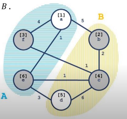
As shown in the figure, the blue and yellow regions are two different connected components. The numbers in square brackets indicate the order of addition to \(A\). Gray nodes are activated nodes, while white nodes are not.
Define \(A_v = \{u \mid \operatorname{pos}(u) < \operatorname{pos}(v)\}\), i.e., the vertices strictly added to \(A\) before \(v\). Let \(E_v\) be the edge set of the induced subgraph of \(E'\) (with vertex set \(A_v \cup\{v\}\)). (Note that it includes vertex \(v\).)
Define the induced cut \(C_v\) as \(C \cap E_v\). \(w(C_v) = \sum_{(i,j) \in C_v} d(i, j)\).
Lemma 1
For any activated vertex \(v\), \(w(A_v, v) \le w(C_v)\).
Proof: By mathematical induction.
For the first activated vertex \(v_0\), by definition, \(w(A_{v_0}, v_0) = w(C_{v_0})\).
For two subsequently activated vertices \(u, v\), assuming \(\operatorname{pos}(v) < \operatorname{pos}(u)\), we have:
\(w(A_u, u) = w(A_v, u) + w(A_u - A_v, u)\)
Also, it is known that:
\(w(A_v, u) \le w(A_v, v)\) and \(w(A_v, v) \le w(C_v)\). Combining these gives:
\(w(A_u, u) \le w(C_v) + w(A_u - A_v, u)\)
Since \(w(A_u - A_v, u)\) contributes to \(w(C_u)\) but not to \(w(C_v)\), and all edge weights are positive, we can deduce:
\(w(A_u,u) \le w(C_u)\)
The lemma is proved by induction.
Since \(\operatorname{pos}(s) < \operatorname{pos}(t)\), and \(s\) and \(t\) are not in the same connected component, \(t\) will be activated. Thus, we can conclude \(w(A_t, t) \le w(C_t) = w(C)\).
P5632【Template】Stoer–Wagner Algorithm
1 2 3 4 5 6 7 8 9 10 11 12 13 14 15 16 17 18 19 20 21 22 23 24 25 26 27 28 29 30 31 32 33 34 35 36 37 38 39 40 41 42 43 44 45 46 47 48 49 50 51 52 53 54 55 56 57 58 59 60 61 62 63 64 65 66 67 68 69 70 71 72 73 74 | |
Complexity Analysis and Optimization
The complexity of the contract operation is \(O(|E| + |V|\log|V|)\).
Since contract is performed \(O(|V|)\) times, the total complexity is \(O(|E||V| + |V|^2\log|V|)\).
Based on experience with Shortest Path, the bottleneck of the algorithm lies in finding the vertex with the maximum weight.
In one contract operation, we need to find the top of the heap \(|V|\) times and incrementally modify weights \(|E|\) times.
A Fibonacci heap can handle \(O(\log|V|)\) top-of-heap lookups and \(O(1)\) incremental weight modifications, theoretically achieving a complexity of \(O(|E| + |V|\log|V|)\). However, due to the large constant factor and high implementation complexity of Fibonacci heaps, their practical value is limited.
(In actual tests, even with O2 optimization, it barely passes due to evaluation fluctuations.)
本页面最近更新:,更新历史
发现错误?想一起完善? 在 GitHub 上编辑此页!
本页面贡献者:OI-wiki
本页面的全部内容在 CC BY-SA 4.0 和 SATA 协议之条款下提供,附加条款亦可能应用