Dominator Tree

Introduction

In 1959, the concept of "domination" was introduced by Reese T. Prosser in a paper on network flows, but no specific algorithm was proposed; it wasn't until 1969 that Edward S. Lowry and C. W. Medlock first presented an effective algorithm. The currently most widely used Lengauer–Tarjan algorithm was proposed by Lengauer and Tarjan in 1979 in a paper.

In the OI community, the concept of the domination tree was first introduced in ZJOI2012 Disaster, where it was also called the "extinction tree"; Chen Sunli also introduced this algorithm in the 2020 National Training Team paper.

Currently, domination trees are not very popular in competitive programming, and related exercises are rare; however, domination trees are widely used in industry, especially in compiler-related fields.

This article will introduce the concept of domination trees and several methods for constructing them.

Dominance Relation

We designate an entry node \(s\) in any directed graph. For a node \(u\), if every path from \(s\) to \(u\) passes through some node \(v\), then we say \(v\) dominates \(u\), or \(v\) is a dominator of \(u\), denoted as \(v\ dom\ u\).

For nodes unreachable from \(s\), discussing their dominance relation is meaningless. Therefore, unless otherwise specified, this article assumes \(s\) can reach every node in the graph.

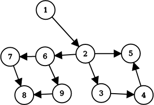
For example, in this directed graph, \(2\) is dominated by \(1\), \(3\) is dominated by \(1, 2\), \(4\) is dominated by \(1, 2, 3\), \(5\) is dominated by \(1, 2\), etc.

Lemmas

In the following lemmas, it is assumed that \(u, v, w\ne s\).

Lemma 1: \(s\) is a dominator of all nodes; every node is a dominator of itself.

Proof: Obviously, any path from \(s\) to \(u\) must pass through both \(s\) and \(u\).

Lemma 2: The dominance relation derived by considering only simple paths is the same as that derived by considering all paths.

Proof: For non-simple paths, let \(S\) be the set of all nodes visited between two visits to some node. If we delete the nodes in \(S\), we can map each non-simple path to a simple path.

In \(S\), nodes that are in the non-simple path but not in the simple path cannot be dominators, because there is at least one simple path from \(s\) to \(u\) that does not include this node; nodes that are in both the simple and non-simple paths only need to be considered in the simple path.

In summary, removing non-simple paths does not affect the dominance relation.

Lemma 3: If \(u\) \(dom\) \(v\) and \(v\) \(dom\) \(w\), then \(u\) \(dom\) \(w\).

Proof: Any path to \(w\) must pass through \(v\), and any path to \(v\) must pass through \(u\). Therefore, any path to \(w\) must pass through \(u\), i.e., \(u \ dom \ w\).

Lemma 4: If \(u \ dom \ v\) and \(v \ dom\ u\), then \(u=v\).

Proof: Assume \(u \ne v\). Then any path reaching \(v\) has already visited \(u\), and any path reaching \(u\) has already visited \(v\), which is a contradiction.

Lemma 5: If \(u \ne v \ne w\), \(u \ dom \ w\) and \(v \ dom \ w\), then either \(u \ dom \ v\) or \(v \ dom \ u\).

Proof: Consider a path \(s \rightarrow \dots \rightarrow u \rightarrow \dots \rightarrow v \rightarrow \dots \rightarrow w\). If \(u\) and \(v\) do not dominate each other, then there must exist a path from \(s\) to \(v\) that does not pass through \(u\), i.e., a path \(s \rightarrow \dots \rightarrow v \rightarrow \dots \rightarrow w\), which contradicts \(u\ dom\ w\).

Computing Dominance Relations

Node Deletion Method

An equivalent conclusion to the definition: If after deleting a certain node from the graph, some nodes become unreachable, then the deleted node dominates those unreachable nodes.

Thus, we can simply try deleting each node and perform DFS. The code complexity is \(O(n^3)\). The core code is provided below.

// Assume there are n nodes in the graph, starting point s = 1
std::bitset<N> vis;
std::vector<int> edge[N];
std::vector<int> dom[N];

void dfs(int u, int del) {
  vis[u] = true;
  for (int v : edge[u]) {
    if (v == del or vis[v]) {
      continue;
    }
    dfs(v, del);
  }
}

void getdom() {
  for (int i = 2; i <= n; ++i) {
    vis.reset();
    dfs(1, i);
    for (int j = 1; j <= n; ++j) {
      if (!vis[j]) {
        dom[j].push_back(i);
      }
    }
  }
}

Data Flow Iteration Method

Data flow iteration is also an uncommon topic in OI. Here is a brief introduction.

Data flow analysis is a concept in compiler theory, used to analyze how data flows along program execution paths. Data flow iteration is a method that sets up equations on nodes of the program's control flow graph and iteratively solves them to obtain data flow values at certain points. Here, we treat the directed graph as a control flow graph.

For this problem, the equation is:

\[ dom(u)=\{u\} \cup \left(\bigcap_{v\in pre(u)}{dom(v)}\right) \]

where \(pre(u)\) is defined as the set of predecessor nodes of \(u\). This equation can be derived from Lemma 3.

In plain language, the set of dominators of a node is the intersection of the dominator sets of all its predecessors, union with itself. We can iteratively update each node's dominator set according to this equation until convergence.

To improve efficiency, we want that during each iteration, as many predecessors as possible of the current node have already been updated. Therefore, we use depth-first ordering to obtain a reverse postorder of the graph and iterate in that order.

Below is a reference implementation of the core code. Note that we need to preprocess each node's predecessor set and the graph's reverse postorder, but this is not the main focus of this article, so no reference implementation is provided here.

std::vector<int> pre[N];  // Predecessors of each node
std::vector<int> ord;     // Reverse postorder of the graph
std::bitset<N> dom[N];
std::vector<int> Dom[N];

void getdom() {
  dom[1][1] = true;
  flag = true;
  while (flag) {
    flag = false;
    for (int u : ord) {
      std::bitset<N> tmp;
      tmp[u] = true;
      for (int v : pre[u]) {
        tmp &= dom[v];
      }
      if (tmp != dom[u]) {
        dom[u] = tmp;
        flag = true;
      }
    }
  }
  for (int i = 2; i <= n; ++i) {
    for (int j = 1; j <= n; ++j) {
      if (dom[i][j]) {
        Dom[i].push_back(j);
      }
    }
  }
}

It is easy to see that the complexity of the above algorithm is \(O(n^2)\).

Dominator Tree

In the previous section, we observed that except for \(s\), a node has at least two dominators: \(s\) and itself.

For any node \(u\), among its dominators (excluding itself), the one closest to \(u\) is called the immediate dominator of \(u\), denoted as \(idom(u) = v\). Clearly, except for \(s\), which has no immediate dominator, every node has a unique immediate dominator.

Consider adding an edge from \(idom(u)\) to \(u\) for every node \(u\) except \(s\). This forms a directed graph with \(n\) nodes and \(n - 1\) edges. According to Lemma 3 and Lemma 4, the dominance relation cannot form cycles, so these edges do not form cycles. Therefore, the resulting graph is actually a tree. We call this tree the dominator tree of the original graph.

Constructing the Dominator Tree

Using dom Sets

Consider the dominator set \(\{s_1, s_2, \dots, s_k\}\) of some node \(u\). There must exist a path \(s \rightarrow \dots \rightarrow s_1 \rightarrow \dots \rightarrow s_2 \rightarrow \dots \rightarrow \dots \rightarrow s_k \rightarrow\dots \rightarrow u\). Clearly, the immediate dominator of \(u\) is \(s_k\). Therefore, the definition of immediate dominator is equivalent to:

For a node \(u\) with dominator set \(S\), if \(v \in S\) satisfies \(\forall w \in S\setminus\{u,v\}, w\ dom \ v\), then \(idom(u)=v\).

Thus, after obtaining each node's dominator set using the previously described algorithm, we can easily determine each node's immediate dominator according to the above definition and construct the dominator tree. Reference code is provided below.

std::bitset<N> dom[N];
std::vector<int> Dom[N];
int idom[N];

void getidom() {
  for (int u = 2; u <= n; ++u) {
    for (int v : Dom[u]) {
      std::bitset<N> tmp = (dom[v] & dom[u]) ^ dom[u];
      if (tmp.count() == 1 and tmp[u]) {
        idom[u] = v;
        break;
      }
    }
  }
  for (int u = 2; u <= n; ++u) {
    e[idom[u]].push_back(u);
  }
}

Special Case: Trees

Obviously, the dominator tree of a tree graph is the tree itself.

Special Case: DAGs

We observe that DAGs have a nice property: solving in topological order ensures that earlier solutions do not affect later ones. We can use this property to quickly construct the dominator tree for a DAG.

Note

It is important to note that the DAG here must have only one starting point. If there are multiple starting points, nodes dominated by multiple starting points would have multiple parents in the dominator tree, making the dominance relation not simply expressible as a tree.

Lemma 6: In a directed graph, \(v\ dom\ u\) if and only if \(\forall w \in pre(u), v\ dom \ w\).

Proof: First, prove sufficiency. Consider any path from \(s\) to \(u\) must pass through some node \(w \in pre(u)\). Since \(v\) dominates \(w\), any path from \(s\) to \(u\) must pass through \(v\), so \(v \ dom \ u\).

Now necessity. If \(\exists w\in pre(u)\) such that \(v\) does not dominate \(w\), then there exists a path \(s \rightarrow \cdots \rightarrow w \rightarrow \cdots \rightarrow u\) that does not pass through \(v\), so \(v\) does not dominate \(u\).

We find that the dominators of \(u\) must be common ancestors of all its predecessors in the dominator tree. Then clearly, the immediate dominator of \(u\) is the LCA of all its predecessors in the dominator tree. Considering that binary lifting for LCA can support adding nodes one by one, the above algorithm is feasible.

Reference implementation:

std::stack<int> sta;
std::vector<int> e[N], g[N], tree[N];  // g is the reverse graph, tree is the dominator tree
int n, s, in[N], tpn[N], dep[N], idom[N];  // n is total nodes, s is start, in is in-degree
int fth[N][17];

void topo(int s) {
  sta.push(s);
  while (!sta.empty()) {
    int u = sta.top();
    sta.pop();
    tpn[++tot] = u;
    for (int v : e[u]) {
      --in[v];
      if (!in[v]) {
        sta.push(v);
      }
    }
  }
}

int lca(int u, int v) {
  if (dep[u] < dep[v]) {
    std::swap(u, v);
  }
  for (int i = 15; i >= 0; --i) {
    if (dep[fth[u][i]] >= dep[v]) {
      u = fth[u][i];
    }
  }
  if (u == v) {
    return u;
  }
  for (int i = 15; i >= 0; --i) {
    if (fth[u][i] != fth[v][i]) {
      u = fth[u][i];
      v = fth[v][i];
    }
  }
  return fth[u][0];
}

void build() {
  topo(s);
  for (int i = 1; i <= n; ++i)
    for (int j = 0; j <= 15; ++j) fth[i][j] = s;
  for (int i = 1; i <= n; ++i) {
    int u = tpn[i];
    if (g[u].size()) {
      int v = g[u][0];
      for (int j = 1, q = g[u].size(); j < q; ++j) {
        v = lca(v, g[u][j]);
      }
      tree[v].push_back(u);
      fth[u][0] = v;
      dep[u] = dep[v] + 1;
      for (int i = 1; i <= 15; ++i) {
        fth[u][i] = fth[fth[u][i - 1]][i - 1];
      }
    }
  }
}

Lengauer–Tarjan Algorithm

The Lengauer–Tarjan algorithm is one of the most famous algorithms for constructing dominator trees. It can compute the dominator tree of a directed graph in \(O(n\alpha(n, m))\) time. This algorithm introduces the concept of semi-dominators and uses them to help find immediate dominators.

Conventions

First, we perform a DFS from \(s\) on the directed graph. The visited nodes and edges form a tree \(T\). We call the traversed edges tree edges and the others non-tree edges. Let \(dfn(u)\) denote the order in which node \(u\) is visited. Define \(u<v\) if and only if \(dfn(u) < dfn(v)\).

Semi-Dominators

The semi-dominator of a node \(u\) is the smallest node \(v\) such that there exists a path from \(v\) to \(u\) where every node except \(u\) and \(v\) is greater than \(u\). Formally, the semi-dominator \(sdom(u)\) is defined as:

\(sdom(u) = \min(v|\exists v=v_0 \rightarrow v_1 \rightarrow\dots \rightarrow v_k = u, \forall 1\le i\le k - 1, v_i > u)\)

We find some useful properties of semi-dominators:

Lemma 7: For any node \(u\), \(sdom(u) < u\).

Proof: According to the definition, \(u\)'s parent \(fa(u)\) in \(T\) also satisfies the condition for being a semi-dominator, and \(fa(u) < u\). Therefore, any node greater than \(u\) cannot be its semi-dominator.

Lemma 8: For any node \(u\), \(idom(u)\) is an ancestor of \(u\) in \(T\).

Proof: The path from \(s\) to \(u\) in \(T\) corresponds to a path in the original graph, and \(idom(u)\) must lie on this path.

Lemma 9: For any node \(u\), \(sdom(u)\) is an ancestor of \(u\) in \(T\).

Proof: Suppose \(sdom(u)\) is not an ancestor of \(u\). Then \(sdom(u)\) cannot have an edge to any node with DFS order greater than or equal to \(u\) (otherwise that node would be in \(sdom(u)\)'s subtree, not another subtree). Contradiction.

Lemma 10: For any node \(u\), \(idom(u)\) is an ancestor of \(sdom(u)\).

Proof: Consider going from \(s\) to \(sdom(u)\) and then following the path in the definition to \(u\). According to the definition, nodes on the path from \(sdom(u)\) to \(u\) do not dominate \(u\), so \(idom(u)\) must be an ancestor of \(sdom(u)\).

Lemma 11: For any nodes \(u \ne v\) such that \(v\) is an ancestor of \(u\), then either \(v\) is an ancestor of \(idom(u)\), or \(idom(u)\) is an ancestor of \(idom(v)\).

Proof: For any node \(w\) between \(v\) and \(idom(v)\), by the definition of immediate dominator, there exists a path from \(s\) to \(idom(v)\) to \(v\) that does not pass through \(w\). Therefore, such \(w\) cannot be \(idom(u)\). Hence, \(idom(u)\) is either a descendant of \(v\) or an ancestor of \(idom(v)\).

Based on the above lemmas, we can derive the following theorem:

Theorem 1: The semi-dominator of a node \(u\) is the minimum among the semi-dominators of all ancestors greater than \(u\) that are either predecessors of \(u\) or reachable from such ancestors. Formally, \(sdom(u)=\min(\{v|\exists v \rightarrow u, v < u \} \cup \{sdom(w) | w > u\ and\ \exists w \rightarrow \dots \rightarrow v \rightarrow u \})\).

Proof: Let \(x\) be the right-hand side of the equation.

First, prove \(sdom(u) \le x\). By Lemma 7, this is equivalent to showing both cases satisfy the semi-dominator condition. The case where \(x\) is a predecessor of \(u\) is obvious. For the second part, consider the path \(x=v_0\rightarrow\dots\rightarrow v_j=w\) from the semi-dominator definition and a path in \(T\) satisfying \(\forall i\in[j, k-1], v_i\ge w > u\): \(w=v_j \rightarrow\dots\rightarrow v_k=v\), concatenated with the edge \(v \rightarrow u\). This constructs a path satisfying the semi-dominator definition.

Next, prove \(sdom(u)\ge x\). Consider the path from the semi-dominator definition: \(sdom(u)=v_0\rightarrow v_1 \rightarrow\dots\rightarrow v_k=u\). Note that \(k=1\) and \(k > 1\) correspond to the two selection methods in the definition. If \(k = 1\), then there is a directed edge \(sdom(u) \rightarrow u\), and by Lemma 7, the proof is done. If \(k>1\), let \(j\) be the smallest integer \(\ge 1\) such that \(v_j\) is an ancestor of \(v_{k-1}\) in \(T\). Since \(k\) satisfies the condition, such \(j\) exists.

Prove that \(v_0 \rightarrow \dots \rightarrow v_j\) is a path satisfying the condition for \(v_j\) to be a semi-dominator, i.e., \(\forall i \in [1, j), v_i>v_j\). If not, let \(i\) be the smallest index such that \(v_i < v_j\). By Lemma 11, \(v_i\) is an ancestor of \(v_j\), contradicting the definition of \(j\). Thus, \(sdom(v_j)\le sdom(u)\). Therefore, \(sdom(u) \le x\), so \(x=sdom(u)\).

Based on Theorem 1, we can compute the semi-dominator for each node. The complexity bottleneck lies in the second case. We can optimize using a weighted union-find set, updating the minimum during path compression.

void dfs(int u) {
  dfn[u] = ++dfc;
  pos[dfc] = u;
  for (int i = h[0][u]; i; i = e[i].x) {
    int v = e[i].v;
    if (!dfn[v]) {
      dfs(v);
      fth[v] = u;
    }
  }
}

int find(int x) {
  if (fa[x] == x) {
    return x;
  }
  int tmp = fa[x];
  fa[x] = find(fa[x]);
  if (dfn[sdm[mn[tmp]]] < dfn[sdm[mn[x]]]) {
    mn[x] = mn[tmp];
  }
  return fa[x];
}

void getsdom() {
  dfs(1);
  for (int i = 1; i <= n; ++i) {
    mn[i] = fa[i] = sdm[i] = i;
  }
  for (int i = dfc; i >= 2; --i) {
    int u = pos[i], res = INF;
    for (int j = h[1][u]; j; j = e[j].x) {
      int v = e[j].v;
      if (!dfn[v]) {
        continue;
      }
      find(v);
      if (dfn[v] < dfn[u]) {
        res = std::min(res, dfn[v]);
      } else {
        res = std::min(res, dfn[sdm[mn[v]]]);
      }
    }
    sdm[u] = pos[res];
    fa[u] = fth[u];
  }
}

Computing Immediate Dominators

Transforming to a DAG

But I still don't know what semi-dominators are for!

Consider adding a directed edge \(sdom(u) \rightarrow u\) to \(T\) for each \(u\). By Lemma 9, the resulting graph \(G\) is a DAG; by Lemma 10, adding these edges does not change the dominance relation. Thus, we transform the original graph into a DAG and can use the previous algorithm.

Using Semi-Dominators

Building extra graphs is inelegant!

Theorem 2: For any node \(u\), if for every node \(v\) on the path from \(sdom(u)\) to \(w\) in \(T\), we have \(sdom(v)\ge sdom(w)\), then \(idom(u) =sdom(u)\).

Proof: By Lemma 10, \(idom(u)\) is either \(sdom(u)\) or an ancestor. So we only need to prove \(sdom(u) \ dom \ u\).

Consider any path \(P\) from \(s\) to \(u\). We need to show \(sdom(u)\) is on \(P\). Let \(v\) be the last node on \(P\) such that \(v<sdom(u)\). If no such \(v\) exists, then \(sdom(u)=idom(u) =s\). Otherwise, let \(w\) be the first node after \(v\) on \(P\) that lies on the DFS tree path from \(sdom(u)\) to \(u\).

We now prove \(sdom(w)\le v <sdom(v)\). Consider the path \(v = v_0 \rightarrow \dots v_k = w\) in \(T\). If the claim is false, then there exists \(i\in[1, k- 1], v_i < w\). Then there must exist some \(j\in [i, k - 1]\) such that \(v_j\) is an ancestor of \(w\). From the choice of \(v\), we have \(sdom(u)\le v_j\), so \(v_j\) is also on the DFS tree path from \(sdom(u)\) to \(u\), contradicting the definition of \(w\). Thus, \(sdom(w)\le v < sdom(v)\). Combined with the theorem condition, we have \(y=sdom(u)\), so path \(P\) contains \(sdom(u)\).

Theorem 3: For any node \(u\), let \(v\) be the node on the path from \(sdom(u)\) to \(u\) in \(T\) with the smallest semi-dominator. Then \(sdom(v)\le sdom(u)\) and \(idom(v) = idom(u)\).

Proof: Since \(u\) itself satisfies the condition for \(v\), we have \(sdom(v)\le sdom(u)\).

Since \(idom(u)\) is an ancestor of \(v\) in \(T\), by Lemma 11, \(idom(u)\) is also an ancestor of \(idom(v)\). So we only need to prove \(idom(v)\) dominates \(u\).

Consider any path \(P\) from \(s\) to \(u\). We need to show \(sdom(u)\) is on \(P\). Let \(x\) be the last node on \(P\) such that \(x<sdom(u)\). If no such \(x\) exists, then \(sdom(u)=idom(u) =s\). Otherwise, let \(y\) be the first node after \(x\) on \(P\) that lies on the DFS tree path from \(sdom(u)\) to \(u\).

Similar to the proof of Theorem 2, we get \(sdom(y) \le x\). By Lemma 10, \(sdom(y)\le x<idom(v) \le sdom(v)\). Now, by the definition of \(v\), \(y\) cannot be a descendant of \(sdom(u)\); on the other hand, \(y\) cannot be both a descendant of \(idom(v)\) and an ancestor of \(v\), because then the path from \(s\) to \(sdom(y)\) along \(P\) to \(y\) and then along the DFS tree to \(v\) would not pass through \(idom(v)\), contradicting the definition of a dominator. Therefore, \(y=idom(v)\), so \(P\) contains \(idom(v)\).

Based on the above two theorems, we can derive the relationship between \(sdom(u)\) and \(idom(u)\).

Let \(v\) be the node on the path from \(sdom(u)\) to \(u\) in \(T\) with the smallest \(sdom(v)\). Then:

\[ idom(u) = \left\{ \begin{aligned} & sdom(u), &\text{if}\ sdom(u) = sdom(v) \\ &idom(v), &\text{otherwise} \end{aligned} \right. \]

We only need to slightly modify the code for computing semi-dominators.

struct E {
  int v, x;
} e[MAX * 4];

int h[3][MAX * 2];

int dfc, tot, n, m, u, v;
int fa[MAX], fth[MAX], pos[MAX], mn[MAX], idm[MAX], sdm[MAX], dfn[MAX],
    ans[MAX];

void add(int x, int u, int v) {
  e[++tot] = {v, h[x][u]};
  h[x][u] = tot;
}

void dfs(int u) {
  dfn[u] = ++dfc;
  pos[dfc] = u;
  for (int i = h[0][u]; i; i = e[i].x) {
    int v = e[i].v;
    if (!dfn[v]) {
      dfs(v);
      fth[v] = u;
    }
  }
}

int find(int x) {
  if (fa[x] == x) {
    return x;
  }
  int tmp = fa[x];
  fa[x] = find(fa[x]);
  if (dfn[sdm[mn[tmp]]] < dfn[sdm[mn[x]]]) {
    mn[x] = mn[tmp];
  }
  return fa[x];
}

void tar(int st) {
  dfs(st);
  for (int i = 1; i <= n; ++i) {
    fa[i] = sdm[i] = mn[i] = i;
  }
  for (int i = dfc; i >= 2; --i) {
    int u = pos[i], res = INF;
    for (int j = h[1][u]; j; j = e[j].x) {
      int v = e[j].v;
      if (!dfn[v]) {
        continue;
      }
      find(v);
      if (dfn[v] < dfn[u]) {
        res = std::min(res, dfn[v]);
      } else {
        res = std::min(res, dfn[sdm[mn[v]]]);
      }
    }
    sdm[u] = pos[res];
    fa[u] = fth[u];
    add(2, sdm[u], u);
    u = fth[u];
    for (int j = h[2][u]; j; j = e[j].x) {
      int v = e[j].v;
      find(v);
      if (sdm[mn[v]] == u) {
        idm[v] = u;
      } else {
        idm[v] = mn[v];
      }
    }
    h[2][u] = 0;
  }
  for (int i = 2; i <= dfc; ++i) {
    int u = pos[i];
    if (idm[u] != sdm[u]) {
      idm[u] = idm[idm[u]];
    }
  }
}

Examples

Luogu P5180【Template】Dominator Tree

You can compute only the dominance relation and record how many nodes each node dominates during the process, or construct the dominator tree and compute the size of each node.

Here is the code for the latter approach.

Reference Code

#include <iostream>
using std::cin;
using std::cout;
constexpr int MAX = 3e5 + 5;
constexpr int INF = 0x5ffffff;

struct E {
  int v, x;
} e[MAX * 4];

int n, m, u, v, tot, dfc;
int ans[MAX], dfn[MAX], pos[MAX], sdm[MAX], idm[MAX], fa[MAX], mn[MAX],
    fth[MAX];
int h[3][MAX * 2];

void add(int x, int u, int v) {
  e[++tot] = {v, h[x][u]};
  h[x][u] = tot;
}

void dfs(int u) {
  dfn[u] = ++dfc;
  pos[dfc] = u;
  for (int i = h[0][u]; i; i = e[i].x) {
    int v = e[i].v;
    if (!dfn[v]) {
      dfs(v);
      fth[v] = u;
    }
  }
}

int find(int x) {
  if (fa[x] == x) {
    return x;
  }
  int tmp = fa[x];
  fa[x] = find(fa[x]);
  if (dfn[sdm[mn[tmp]]] < dfn[sdm[mn[x]]]) {
    mn[x] = mn[tmp];
  }
  return fa[x];
}

void tar(int st) {
  dfs(st);
  for (int i = 1; i <= n; ++i) {
    mn[i] = fa[i] = sdm[i] = i;
  }
  for (int i = dfc; i >= 2; --i) {
    int u = pos[i], res = INF;
    for (int j = h[1][u]; j; j = e[j].x) {
      int v = e[j].v;
      if (!dfn[v]) {
        continue;
      }
      find(v);
      if (dfn[v] < dfn[u]) {
        res = std::min(res, dfn[v]);
      } else {
        res = std::min(res, dfn[sdm[mn[v]]]);
      }
    }
    sdm[u] = pos[res];
    fa[u] = fth[u];
    add(2, sdm[u], u);
    u = fth[u];
    for (int j = h[2][u]; j; j = e[j].x) {
      int v = e[j].v;
      find(v);
      if (u == sdm[mn[v]]) {
        idm[v] = u;
      } else {
        idm[v] = mn[v];
      }
    }
    h[2][u] = 0;
  }
  for (int i = 2; i <= dfc; ++i) {
    int u = pos[i];
    if (idm[u] != sdm[u]) {
      idm[u] = idm[idm[u]];
    }
  }
  for (int i = dfc; i >= 2; --i) {
    ++ans[pos[i]];
    ans[idm[pos[i]]] += ans[pos[i]];
  }
  ++ans[1];
}

int main() {
  cin >> n >> m;
  for (int i = 1; i <= m; ++i) {
    cin >> u >> v;
    add(0, u, v);
    add(1, v, u);
  }
  tar(1);
  for (int i = 1; i <= n; ++i) {
    cout << ans[i] << ' ';
  }
}

ZJOI2012 Disaster

Compute the dominator tree on the DAG and then compute node sizes.

Reference Code

#include <iostream>
#include <stack>
#include <vector>

using std::cin;
using std::cout;
using std::stack;
using std::vector;

constexpr int MAX = 65536;
int n, x, tot;
int d[MAX], w[MAX], siz[MAX], p[MAX], f[MAX][17];
vector<int> e[MAX], g[MAX], h[MAX];
stack<int> s;

void topo() {
  s.push(0);
  for (int i = 1; i <= n; ++i) {
    if (!w[i]) {
      e[0].push_back(i);
      g[i].push_back(0);
      ++w[i];
    }
  }
  while (!s.empty()) {
    int x = s.top();
    s.pop();
    p[++tot] = x;
    for (int i : e[x]) {
      --w[i];
      if (!w[i]) {
        s.push(i);
      }
    }
  }
}

int lca(int u, int v) {
  if (d[u] < d[v]) {
    std::swap(u, v);
  }
  for (int i = 15; i >= 0; --i) {
    if (d[f[u][i]] >= d[v]) {
      u = f[u][i];
    }
  }
  if (u == v) {
    return u;
  }
  for (int i = 15; i >= 0; --i) {
    if (f[u][i] != f[v][i]) {
      u = f[u][i];
      v = f[v][i];
    }
  }
  return f[u][0];
}

void dfs(int x) {
  siz[x] = 1;
  for (int i : h[x]) {
    dfs(i);
    siz[x] += siz[i];
  }
}

void build() {
  for (int i = 2; i <= n + 1; ++i) {
    int x = p[i], y = g[x][0];
    for (int j = 1, q = g[x].size(); j < q; ++j) {
      y = lca(y, g[x][j]);
    }
    h[y].push_back(x);
    d[x] = d[y] + 1;
    f[x][0] = y;
    for (int i = 1; i <= 15; ++i) {
      f[x][i] = f[f[x][i - 1]][i - 1];
    }
  }
}

int main() {
  cin >> n;
  for (int i = 1; i <= n; ++i) {
    while (true) {
      cin >> x;
      if (!x) {
        break;
      }
      e[x].push_back(i);
      g[i].push_back(x);
      ++w[i];
    }
  }
  topo();
  build();
  dfs(0);
  for (int i = 1; i <= n; ++i) {
    cout << siz[i] - 1 << '\n';
  }
  return 0;
}

---

本页面最近更新：，更新历史
发现错误？想一起完善？ 在 GitHub 上编辑此页！
本页面贡献者：OI-wiki
本页面的全部内容在 CC BY-SA 4.0 和 SATA 协议之条款下提供，附加条款亦可能应用