Inclusion–Exclusion Principle

Introduction

Introductory Example

Suppose there are \(10\) students who like math, \(15\) students who like Chinese, and \(21\) students who like programming. How many students like at least one of these subjects?

Is it \(10+15+21=46\)? No, because some students may like both math and Chinese, or Chinese and programming, or even all three.

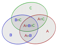
For convenience, let the sets of students who like Chinese, math, and programming be denoted by \(A,B,C\) respectively. Then the total number of students is \(|A\cup B\cup C|\). As mentioned earlier, if we simply add the sizes of these three sets \(|A|,|B|,|C|\), some elements will be counted multiple times. Therefore, we need to subtract \(|A\cap B|,|B\cap C|,|C\cap A|\). However, this will over-subtract a small portion, so we need to add back \(|A\cap B\cap C|\). That is,

\[ |A\cup B\cup C|=|A|+|B|+|C|-|A\cap B|-|B\cap C|-|C\cap A|+|A\cap B\cap C| \]

Inclusion–exclusion principle - Venn diagram example

Generalizing the above problem leads to the well-known inclusion–exclusion principle.

Definition

Let the elements in \(U\) have \(n\) different properties, and the \(i\)-th property is called \(P_i\). The set of elements possessing property \(P_i\) is \(S_i\). Then

\[ \begin{aligned} \left|\bigcup_{i=1}^{n}S_i\right|=&\sum_{i}|S_i|-\sum_{i<j}|S_i\cap S_j|+\sum_{i<j<k}|S_i\cap S_j\cap S_k|-\cdots\\ &+(-1)^{m-1}\sum_{a_i<a_{i+1} }\left|\bigcap_{i=1}^{m}S_{a_i}\right|+\cdots+(-1)^{n-1}|S_1\cap\cdots\cap S_n| \end{aligned} \]

i.e.,

\[ \left|\bigcup_{i=1}^{n}S_i\right|=\sum_{m=1}^n(-1)^{m-1}\sum_{a_i<a_{i+1} }\left|\bigcap_{i=1}^mS_{a_i}\right| \]

Proof

For each element, compute the number of times it appears using the binomial theorem. For an element \(x\), suppose it appears in the sets \(T_1,T_2,\cdots,T_m\). Then its count is

\[ \begin{aligned} Cnt=&|\{T_i\}|-|\{T_i\cap T_j|i<j\}|+\cdots+(-1)^{k-1}\left|\left\{\bigcap_{i=1}^{k}T_{a_i}|a_i<a_{i+1}\right\}\right|\\ &+\cdots+(-1)^{m-1}|\{T_1\cap\cdots\cap T_m\}|\\ =&\dbinom{m}{1}-\dbinom{m}{2}+\cdots+(-1)^{m-1}\dbinom{m}{m}\\ =&\dbinom{m}{0}-\sum_{i=0}^m(-1)^i\dbinom{m}{i}\\ =&1-(1-1)^m=1 \end{aligned} \]

Thus, each element appears exactly once, so the sum equals the size of the union. Q.E.D.

Complement

For the union of sets under the universal set \(U\), the inclusion–exclusion principle can be used. The intersection of sets can be obtained by subtracting the union of complements from the universal set:

\[ \left|\bigcap_{i=1}^{n}S_i\right|=|U|-\left|\bigcup_{i=1}^n\overline{S_i}\right| \]

The right-hand side can be computed using inclusion–exclusion.

Readers familiar with inclusion–exclusion may already know the above content and are more interested in its applications.

Next, we present three examples of varying difficulty to demonstrate the application of the inclusion–exclusion principle.

Counting Non-negative Integer Solutions to Indefinite Equations

Given the indefinite equation \(\sum_{i=1}^nx_i=m\) and \(n\) constraints \(x_i\leq b_i\), where \(m,b_i \in \mathbb{N}\). Find the number of non-negative integer solutions.

Without Constraints

Without the constraints \(x_i\leq b_i\), the number of non-negative integer solutions to \(\sum_{i=1}^nx_i=m\) is \(\dbinom{m+n-1}{n-1}\).

Brief proof: stars and bars method.

Imagine distributing \(m\) balls into \(n\) boxes, allowing some boxes to be empty. This problem cannot be directly solved using combinations.

We add \(n-1\) additional balls, so the problem becomes choosing \(n-1\) balls from a sequence of \(m+n-1\) balls. These \(n-1\) balls divide the sequence into \(n\) segments, corresponding to the \(n\) boxes. The number of ways to choose \(n-1\) balls from \(m+n-1\) balls is \(\dbinom{m+n-1}{n-1}\).

Inclusion–Exclusion Model

Now we abstract the inclusion–exclusion model:

Universal set \(U\): non-negative integer solutions to \(\sum_{i=1}^nx_i=m\).
Elements: variables \(x_i\).
Properties: the condition \(x_i\) satisfies, i.e., \(x_i\leq b_i\).

Goal: the size of the set where all variables satisfy their corresponding properties, i.e., \(|\bigcap_{i=1}^nS_i|\).

This can be solved using \(\left|\bigcap_{i=1}^{n}S_i\right|=|U|-\left|\bigcup_{i=1}^n\overline{S_i}\right|\). \(|U|\) can be computed via combinations, and the latter part is expanded using inclusion–exclusion.

The problem reduces to computing the size of intersections of some \(\overline{S_{a_i}}\). Consider the meaning of \(\overline{S_{a_i} }\): it represents the number of solutions where \(x_{a_i}\geq b_{a_i}+1\). The intersection means satisfying all these conditions simultaneously. Thus, in the indefinite equation corresponding to this intersection, some variables have lower bounds, while others have no restrictions.

Can we eliminate these lower bounds? Since we require non-negative integer solutions and some variables have lower bounds greater than \(0\), we can subtract these lower bounds to reduce them to \(0\), i.e., remove the lower bounds. Therefore, for

\[ \left|\bigcap_{a_i<a_{i+1} }^{1\leq i\leq k}S_{a_i}\right| \]

the indefinite equation becomes

\[ \sum_{i=1}^nx_i=m-\sum_{i=1}^k(b_{a_i}+1) \]

This can also be computed via combinations. The array \(a\) of length \(k\) essentially enumerates subsets.

HAOI2008 Coin Shopping

There are 4 types of coins, with the \(i\)-th type having denomination \(C_i\). There are \(n\) queries. Each query gives the quantity \(D_i\) for each coin type and a price \(S\). Find the number of payment methods.

\(n\leq 10^3,S\leq 10^5\).

Using a knapsack approach, the complexity would be \(O(4nS)\), which is unacceptable. The key feature of this problem is that there are only four coin types. Abstractly, we need to find the number of non-negative integer solutions to \(\sum_{i=1}^4C_ix_i=S,x_i\leq D_i\).

Using the same inclusion–exclusion approach, the property for \(x_i\) is \(x_i\leq D_i\). Applying the inclusion–exclusion formula, we finally need to solve

\[ \sum_{i=1}^4C_ix_i=S-\sum_{i=1}^kC_{a_i}(D_{a_i}+1) \]

which is an unbounded knapsack problem. This can be preprocessed. Including queries, the total complexity is \(O(4S+2^4n)\).

Code Implementation

#include <iostream>
using namespace std;
constexpr long long S = 1e5 + 5;
long long c[5], d[5], n, s;
long long f[S];

int main() {
  cin.tie(nullptr)->sync_with_stdio(false);
  cin >> c[1] >> c[2] >> c[3] >> c[4] >> n;
  f[0] = 1;
  for (long long j = 1; j <= 4; j++)
    for (long long i = 1; i < S; i++)
      if (i >= c[j]) f[i] += f[i - c[j]];  // f[i]: number of coin combinations for price i
  for (long long k = 1; k <= n; k++) {
    cin >> d[1] >> d[2] >> d[3] >> d[4] >> s;
    long long ans = 0;
    for (long long i = 1; i < 16;
         i++) {  // Inclusion-exclusion principle, since there are 4 types of items, loop from 1 to 2^4-1=15
      long long m = s, bit = 0;
      for (long long j = 1; j <= 4; j++) {
        if ((i >> (j - 1)) % 2 == 1) {
          m -= (d[j] + 1) * c[j];
          bit++;
        }
      }
      if (m >= 0) ans += (bit % 2 * 2 - 1) * f[m];
    }
    cout << f[s] - ans << '\n';
  }
  return 0;
}

Complete Graph Subgraph Coloring Problem

The previous three problems are direct applications of inclusion–exclusion. This problem requires reverse analysis using inclusion–exclusion.

Complete Graph Subgraph Coloring Problem

A and B enjoy coloring graphs (not necessarily connected) with the rule that adjacent vertices must have the same color. Today, A and B play a game on an \(n\)-vertex complete graph \(G=(V,E)\). They define an evaluation function \(F(S)\), where \(S\) is an edge set, \(S\subseteq E\). \(F(S)\) is the total number of ways to color the graph \(G'=(V,S)\) with \(m\) colors. Another rule is: if \(|S|\) is odd, A's score increases by \(F(S)\); otherwise, B's score increases by \(F(S)\). Find the difference between A's and B's scores.

Mathematical Form

The scoring difference is the symmetric difference between odd and even, which can be expressed using powers of \(-1\) as coefficients. We compute

\[ Ans=\sum_{S\subseteq E}(-1)^{|S|-1}F(S) \]

Inclusion–Exclusion Model

Adjacent vertices having the same color is treated as a property. Here, we first ignore the coloring rule and assume we directly color the graph with \(m\) colors. For a graph \(G'=(V,S)\), treat it as an element. The property \(x_i=x_j\) means vertices \(i\) and \(j\) have the same color (note: it does not require an edge between \(i\) and \(j\)).

The set corresponding to property \(x_i=x_j\) is defined as \(Q_{i,j}\), meaning all coloring schemes of \(G'\) satisfying this property. The size of the set is the number of coloring schemes satisfying this property, and elements within the set correspond to colored graphs \(G'\) satisfying the property.

Returning to the problem, "adjacent vertices must have the same color" can be interpreted as the intersection of several \(Q\) sets. Thus,

\[ F(S)=\left|\bigcap_{(i,j)\in S}Q_{i,j}\right| \]

The right-hand side means the number of coloring schemes where for every edge \((i,j)\) in \(S\), \(x_i=x_j\) holds, i.e., \(F(S)\).

This resembles inclusion–exclusion. Since inclusion–exclusion does not naturally handle pairs, we map all edges \((i,j)\) to \(T=\frac{n(n+1)}{2}\) integers. Suppose \((i,j)\) is mapped to \(k,1\leq k\leq T\), and \(Q_{i,j}\) is mapped to \(Q_k\). Then property \(x_i=x_j\) is defined as \(P_k\).

Also, \(S\) can be represented as a set of \(k\) values, i.e., \(S\iff K=\{k_1,k_2,\cdots,k_m\}\) (i.e., we establish an equivalence between edge sets and integer sets).

And \(E\) corresponds to the set \(M=\left\{1,2,\cdots,\frac{n(n+1)}{2}\right\}\). Thus,

\[ F(S)\iff F(\{ {k_i}\})=\left|\bigcap_{k_i}Q_{k_i}\right| \]

Reverse Analysis

Expanding the desired expression:

\[ \begin{aligned} Ans &= \sum_{K\subseteq M}(-1)^{|K|-1}\left|\bigcap_{k_i\in K}Q_{k_i}\right|\\ &= \sum_{i}|Q_i|-\sum_{i<j}|Q_i\cap Q_j|+\sum_{i<j<k}|Q_i\cap Q_j\cap Q_k|-\cdots+(-1)^{T-1}\left|\bigcap_{i=1}^TQ_i\right| \end{aligned} \]

This is the expanded form of inclusion–exclusion. Reverse derivation yields

\[ Ans=\left|\bigcup_{i=1}^TQ_i\right| \]

Consider the meaning of the right-hand side: it suffices to satisfy any condition from \(1\) to \(T\), i.e., coloring schemes where there exist two vertices (not necessarily adjacent) with the same color! The total number of coloring schemes is \(U\), and clearly \(|U|=m^n\). Converting to the complement, we seek the number of coloring schemes where all vertices have distinct colors, i.e., \(A_m^n=\frac{m!}{(m-n)!}\). Therefore,

\[ Ans=m^n-A_m^n \]

To solve this problem, we first abstract the mathematical form, then start from the most informative condition—the definition of \(F(S)\)—and transform it into set intersections and unions. Then we convert the expression into an inclusion–exclusion form and reverse derive the final result. This problem demonstrates the inverse application of inclusion–exclusion.

Inclusion–Exclusion in Number Theory

Inclusion–exclusion can elegantly solve some number theory problems.

Counting Pairs with GCD Equal to k

Consider the following problem:

Counting Pairs with GCD Equal to \(k\)

Let \(1 \le x, y \le N\), and \(f(k)\) denote the number of ordered pairs \((x, y)\) with \(\gcd(x, y) = k\). Find \(f(1)\) to \(f(N)\).

This problem can be solved using Euler's totient function or Möbius inversion, but inclusion–exclusion is simpler.

By inclusion–exclusion, first find all pairs where \(k\) is a common divisor, then subtract all pairs where a multiple of \(k\) is the common divisor. The remaining pairs are those where \(k\) is the greatest common divisor. That is, \(f(k)=\) number of pairs with \(k\) as a common divisor \(-\) number of pairs with a multiple of \(k\) as a common divisor.

Further, the number of pairs with a multiple of \(k\) as a common divisor equals the sum of the number of pairs with each multiple of \(k\) as the greatest common divisor. Thus, we can write:

\[ f(k)= \lfloor (N/k) \rfloor ^2 - \sum_{i=2}^{i*k \le N} f(i*k) \]

Since for \(k>N/2\), we can directly compute \(f(k)= \lfloor (N/k) \rfloor ^2\), we can compute backwards from \(f(N)\) to \(f(1)\). Thus, we solve the problem using inclusion–exclusion.

for (long long k = N; k >= 1; k--) {
  f[k] = (N / k) * (N / k);
  for (long long i = k + k; i <= N; i += k) f[k] -= f[i];
}

The time complexity of the above method is \(O( \sum_{i=1}^{N} N/i)=O(N \sum_{i=1}^{N} 1/i)=O(N \log N)\).

Here are three similar problems for practice:

Deriving Euler's Totient Function via Inclusion–Exclusion

Consider the following problem:

Euler's Totient Function Formula

Find Euler's totient function \(\varphi(n)\). Here \(\varphi(n)=|\{1\leq x\leq n|\gcd(x,n)=1\}|\).

Direct computation is \(O(n\log n)\), linear sieve is \(O(n)\), and Du's sieve is \(O(n^{\frac{2}{3}})\) (though for an introductory number theory problem, why mention Du's sieve?). Next, we derive Euler's totient function formula using inclusion–exclusion.

To determine if two numbers are coprime, first factorize:

\[ n=\prod_{i=1}^k{p_i}^{c_i} \]

Then we require that for any \(p_i\), \(x\) is not a multiple of \(p_i\), i.e., \(p_i\nmid x\). Treat this as a property, with corresponding set \(S_i\). Thus,

\[ \varphi(n)=\left|\bigcap_{i=1}^kS_i\right|=|U|-\left|\bigcup_{i=1}^k\overline{S_i}\right| \]

The universal set size is \(|U|=n\), and \(\overline{S_i}\) represents the set where \(p_i\mid x\), so clearly \(|\overline{S_i}|=\frac{n}{p_i}\). From this, we derive

\[ \left|\bigcap_{a_i<a_{i+1}}S_{a_i}\right|=\frac{n}{\prod p_{a_i}} \]

Thus,

\[ \begin{aligned} \varphi(n)&=n-\sum_{i}\frac{n}{p_i}+\sum_{i<j}\frac{n}{p_ip_j}-\cdots+(-1)^k\frac{n}{p_1p_2 \cdots p_k}\\ &=n\left(1-\frac{1}{p_1}\right)\left(1-\frac{1}{p_2}\right)\cdots\left(1-\frac{1}{p_k}\right)\\ &=n\prod_{i=1}^k\left(1-\frac{1}{p_i}\right) \end{aligned} \]

This is the mathematical expression for Euler's totient function.

Generalization of Inclusion–Exclusion

Inclusion–exclusion is commonly used for counting sets. For functions \(f(S),g(S)\) on two sets, if

\[ f(S)=\sum_{T\subseteq S}g(T) \]

then

\[ g(S)=\sum_{T\subseteq S}(-1)^{|S|-|T|}f(T) \]

Proof

We start from the right-hand side:

\[ \begin{aligned} &\sum_{T\subseteq S}(-1)^{|S|-|T|}f(T)\\ =&\sum_{T\subseteq S}(-1)^{|S|-|T|}\sum_{Q\subseteq T}g(Q)\\ =&\sum_{Q}g(Q)\sum_{Q\subseteq T\subseteq S}(-1)^{|S|-|T|}\\ \end{aligned} \]

We notice the latter summation is independent of \(Q\), so we factor out \(Q\):

\[ =\sum_{Q}g(Q)\sum_{T\subseteq (S\setminus Q)}(-1)^{|S\setminus Q|-|T|} \]

Define a function on sets \(F(P)=\sum_{T\subseteq P}(-1)^{|P|-|T|}\), and simplify:

\[ \begin{aligned} F(P)&=\sum_{T\subseteq P}(-1)^{|P|-|T|}\\ &=\sum_{i=0}^{|P|}\dbinom{|P|}{i}(-1)^{|P|-i}=\sum_{i=0}^{|P|}\dbinom{|P|}{i}1^i(-1)^{|P|-i}\\ &=(1-1)^{|P|}=0^{|P|} \end{aligned} \]

Thus, the original expression becomes

\[ \sum_{Q}g(Q)\sum_{T\subseteq (S\setminus Q)}(-1)^{|S\setminus Q|-|T|}=\sum_{Q}g(Q)F(S\setminus Q)=\sum_{Q}g(Q)\cdot 0^{|S\setminus Q|} \]

Analysis shows that only when \(|S\setminus Q|=0\) does \(0^0=1\), which occurs when \(Q=S\), contributing \(g(S)\) to the answer. Otherwise, \(0^{|S\setminus Q|}=0\), contributing nothing. Hence,

\[ \sum_{Q}g(Q)\cdot 0^{|S\setminus Q|}=g(S) \]

Thus, the proof is complete.

Corollary

This form also has a corollary. Under the universal set \(U\), for functions \(f(S),g(S)\), if

\[ f(S)=\sum_{S\subseteq T}g(T) \]

then

\[ g(S)=\sum_{S\subseteq T}(-1)^{|T|-|S|}f(T) \]

This corollary is essentially the complement form, with a similar proof.

DAG Counting

Count the number of directed acyclic graphs (DAGs) with \(n\) labeled vertices, modulo \(10^9+7\). \(n\leq 5\times 10^3\).

Direct DP

Consider DP. Define \(f[i,j]\) as the number of DAGs with \(i\) vertices and exactly \(j\) vertices with in-degree \(0\). Suppose after removing these \(j\) vertices, there are \(k\) vertices with in-degree \(0\). Before removal, these \(k\) vertices must have edges to at least some of the \(j\) vertices, giving \(2^j-1\) possibilities. The \(j\) vertices can also have edges to the remaining vertices arbitrarily, giving \(2^{i-j-k}\) possibilities. Thus,

\[ f[i,j]=\binom{i}{j}\sum_{k=1}^{i-j}(2^j-1)^k2^{(i-j-k)j}f[i-j,k] \]

Computing this has complexity \(O(n^3)\).

Relaxing Constraints

The above DP definition is too strict: exactly \(j\) vertices with in-degree \(0\). We can relax it to at least \(j\) vertices with in-degree \(0\). Define \(f[i]\) as the number of DAGs with \(i\) vertices. Direct inclusion–exclusion can be applied. Consider the chosen \(j\) vertices: they can have arbitrary edges to the remaining \(i-j\) vertices, i.e., \(\left(2^{i-j}\right)^j=2^{(i-j)j}\) possibilities:

\[ f[i]=\sum_{j=1}^i(-1)^{j-1}\binom{i}{j}2^{(i-j)j}f[i-j] \]

Computing this has complexity \(O(n^2)\).

Min-max Inclusion–Exclusion

For a sequence \(\{x_i\}\) satisfying a total order and whose elements are additive, let its length be \(n\), and let \(S=\{1,2,3,\cdots,n\}\). Then:

\[ \max_{i\in S}{x_i}=\sum_{T\subseteq S}{(-1)^{|T|-1}\min_{j\in T}{x_j}} \]

\[ \min_{i\in S}{x_i}=\sum_{T\subseteq S}{(-1)^{|T|-1}\max_{j\in T}{x_j}} \]

Proof: Consider a mapping to the general inclusion–exclusion principle. For \(x\in S\), suppose \(x\) is the \(k\)-th smallest element. Define a mapping \(f:x\mapsto \{1,2,\cdots,k\}\). Clearly, this is a bijection.

It is easy to see that for \(x,y\in S\), \(f(\min(x,y))=f(x)\cap f(y)\) and \(f(\max(x,y))=f(x)\cup f(y)\). Thus,

\[ \begin{aligned} \left|f\left(\max_{i\in S}{x_i}\right)\right| &= \left| \bigcup_{i\in S} f(x_i) \right|\\ &= \sum_{T\subseteq S}(-1)^{|T|-1} \left|\bigcap_{j\in T}f(x_j)\right|\\ &= \sum_{T\subseteq S}(-1)^{|T|-1} \left|f\left(\min_{j\in T}{x_j}\right)\right|\\ \end{aligned} \]

Then map \(\left|f\left(\max_{i\in S}{x_i}\right)\right|\) back to \(\max_{i\in S}{x_i}\), and similarly for \(\min\).

Q.E.D.

You might think this formula is trivial since the maximum can be directly computed. The importance of min-max inclusion–exclusion lies in its validity for expectations:

\[ E\left(\max_{i\in S}{x_i}\right)=\sum_{T\subseteq S}{(-1)^{|T|-1}E\left(\min_{j\in T}{x_j} \right)} \]

\[ E\left(\min_{i\in S}{x_i}\right)=\sum_{T\subseteq S}{(-1)^{|T|-1}E\left(\max_{j\in T}{x_j} \right)} \]

Proof: Consider a method to compute expectation:

\[ E\left(\max_{i\in S}{x_i}\right)=\sum_{y}{P(y=x)\max_{j\in S}{y_j}} \]

where \(y\) is a sequence of length \(n\).

Apply the previous formula to the \(\max\):

\[ \begin{aligned}E\left(\max_{i\in S}{x_i}\right)&=\sum_{y}{P(y=x)\max_{j\in S}{y_j}}\\ &=\sum_{y}{P(y=x)\sum_{T\subseteq S}{(-1)^{|T|-1}\min_{j\in T}{y_j}}} \end{aligned} \]

Swap summation order:

\[ \begin{aligned}E\left(\max_{i\in S}{x_i}\right) &=\sum_{y}{P(y=x)\sum_{T\subseteq S}{(-1)^{|T|-1}\min_{j\in T}{y_j}}}\\ &=\sum_{T\subseteq S}{(-1)^{|T|-1}\sum_y{P(y=x)\min_{j\in T}{y_j}}}\\ &=\sum_{T\subseteq S}{(-1)^{|T|-1}E\left(\min_{j\in T}{y_j}\right)} \end{aligned} \]

Similarly for \(\min\).

Q.E.D.

There is a stronger version:

\[ \underset{i\in S}{\operatorname{kthmax}{x_i}}=\sum_{T\subseteq S}{(-1)^{|T|-k}\dbinom {|T|-1}{k-1}\min_{j\in T}{x_j}} \]

\[ \underset{i\in S}{\operatorname{kthmin}{x_i}}=\sum_{T\subseteq S}{(-1)^{|T|-k}\dbinom {|T|-1}{k-1}\max_{j\in T}{x_j}} \]

\[ E\left(\underset{i\in S}{\operatorname{kthmax}{x_i}}\right)=\sum_{T\subseteq S}{(-1)^{|T|-k}\dbinom {|T|-1}{k-1}E\left(\min_{j\in T}{x_j}\right)} \]

\[ E\left(\underset{i\in S}{\operatorname{kthmin}{x_i}}\right)=\sum_{T\subseteq S}{(-1)^{|T|-k}\dbinom {|T|-1}{k-1}E\left(\max_{j\in T}{x_j}\right)} \]

Define \(\dbinom nm=0\) if \(n< m\).

Proof: Without loss of generality, assume \(\forall 1\le i<n,x_i\le x_{i+1}\). Then:

\[ \begin{aligned} \sum_{T\subseteq S}{(-1)^{|T|-k}\dbinom {|T|-1}{k-1}\min_{j\in T}{x_j}} &=\sum_{i\in S}{x_i\sum_{T\subseteq S}{(-1)^{|T|-k}\dbinom {|T|-1}{k-1}\left[x_i=\min_{j\in T}{x_j} \right]}}\\ &=\sum_{i\in S}{x_i\sum_{j=k}^n{\dbinom {n-i}{j-1}\dbinom {j-1}{k-1}(-1)^{j-k}}} \end{aligned} \]

Using the combinatorial identity \(\dbinom ab\dbinom bc=\dbinom ac\dbinom {a-c}{b-c}\), we have:

\[ \begin{aligned} \sum_{T\subseteq S}{(-1)^{|T|-k}\dbinom {|T|-1}{k-1}\min_{j\in T}{x_j}} &=\sum_{i\in S}{x_i\sum_{j=k}^n{\dbinom {n-i}{j-1}\dbinom {j-1}{k-1}(-1)^{j-k}}}\\ &=\sum_{i\in S}{x_i\sum_{j=k}^n{\dbinom {n-i}{k-1}\dbinom {n-i-k+1}{j-k}(-1)^{j-k}}}\\ &=\sum_{i\in S}{\dbinom {n-i}{k-1}x_i\sum_{j=k}^n{\dbinom {n-i-k+1}{j-k}(-1)^{j-k}}}\\ &=\sum_{i\in S}{\dbinom {n-i}{k-1}x_i\sum_{j=0}^{n-i-k+1}{\dbinom {n-i-k+1}j(-1)^{j}}} \end{aligned} \]

When \(i=n-k+1\):

\[ \dbinom {n-i}{k-1}\sum_{j=0}^{n-i-k+1}{\dbinom {n-i-k+1}j(-1)^{j}}=1 \]

Otherwise:

\[ \dbinom {n-i}{k-1}\sum_{j=0}^{n-i-k+1}{\dbinom {n-i-k+1}j(-1)^{j}}=0 \]

Thus:

\[ \sum_{i\in S}{\dbinom {n-i}{k-1}x_i\sum_{j=0}^{n-i-k+1}{\dbinom {n-i-k+1}j(-1)^{j}}}=\underset{i\in S}{\operatorname{kthmax}}{x_i} \]

The remaining three are similar.

Q.E.D.

From min-max inclusion–exclusion, we also have:

\[ \underset{i\in S}{\operatorname{lcm}}{x_i}=\prod_{T\subseteq S}{\left(\gcd_{j\in T}{x_j} \right)^{(-1)^{|T|-1}}} \]

Because \(\operatorname{lcm},\gcd,a^{1},a^{-1}\) correspond to \(\max,\min,+,-\) respectively, i.e., min-max inclusion–exclusion applied to exponents, so it holds.

PKUWC2018 Random Walk

Given a tree with \(n\) vertices, you start from \(x\) and at each step randomly choose an edge adjacent to the current vertex to traverse.

There are \(Q\) queries. Each query gives a set \(S\). Find the expected number of steps until every vertex in \(S\) has been visited at least once.

Specifically, vertex \(x\) (the starting point) is considered visited from the beginning.

Modulo \(998244353\).

\(1\le n\le 18,1\le Q\le 5000,1\le |S|\le n\).

The expected number of steps is the expected time. Let the random variable \(x_i\) be the first time vertex \(i\) is visited. We seek

\[ E\left(\max_{i\in S}x_i\right) \]

Using min-max inclusion–exclusion:

\[ E\left(\max_{i\in S}x_i\right) =E\left(\sum_{T\subseteq S}(-1)^{|T|-1}\min_{i\in T}x_i\right) =\sum_{T\subseteq S}(-1)^{|T|-1}E\left(\min_{i\in T}x_i\right) \]

For a set \(T\in[n]\), compute \(F(T)=E(\min_{i\in T}x_i)\).

\(E(\min_{i\in T}x_i)\) is the expected time to first visit any vertex in \(T\). Let \(f(i)\) be the expected time starting from vertex \(i\) to first visit any vertex in \(T\).

For \(i\in T\), \(f(i)=0\).
For \(i\notin T\), \(f(i)=1+\frac{1}{\text{deg}(i)}\sum_{(i,j)\in E}f(j)\).

Direct Gaussian elimination would be \(O(n^3)\). Computing \(F(T)\) for each \(T\) would be \(O(2^nn^3)\), unacceptable. We use tree elimination.

Let the root be \(1\), and \(p_u\) be the parent of vertex \(u\). For leaf \(i\), \(f(i)\) only depends on its parent (or \(f(i)=0\), which is simpler). Thus, we can express \(f(i)=A_i+B_if(p_i)\), where \(A_i,B_i\) can be computed quickly.

For non-leaf \(i\), consider its children \(j_1,\cdots,j_k\). Since \(f(j_e)=A_{j_e}+B_{j_e}f(i)\), we have

\[ f(i)=1+\frac{1}{\deg(i)}\sum_{e=1}^k\left(A_{j_e}+B_{j_e}f(i)\right)+\frac{f(p_i)}{\deg(i)} \]

Rearranging:

\[ f(i)=\frac{\deg(i)+\sum_{e=1}^kA_{j_e}}{\deg(i)-\sum_{e=1}^kB_{j_e}}+ \frac{f(p_i)}{\deg(i)-\sum_{e=1}^kB_{j_e}} \]

Thus, \(f(i)\) is also expressed as \(A_i+B_if(p_i)\). This can be propagated up to the root. The root has no parent, so

\[ f(1)=\frac{\deg(1)+\sum_{e=1}^kA_{j_e}}{\deg(1)-\sum_{e=1}^kB_{j_e}} \]

Solving this equation gives \(f(1)\), and then propagating downwards gives \(f(i)\) for each vertex. Then \(F(T)=f(x)\). Time complexity \(O(n)\).

Thus, for each \(T\), we compute \(F(T)\) in \(O(2^nn)\) total time.

Returning to inclusion–exclusion, \(E(\max_{i\in S}x_i)=\sum_{T\subseteq S}(-1)^{|T|-1}F(T)\).

Let \(F'(T)=(-1)^{|T|-1}F(T)\). Then \(E(\max_{i\in S}x_i)=\sum_{T\subseteq S}F'(T)\). Thus, we can use FMT (also called subset prefix sum, or FWT or transform) to compute \(E(\max_{i\in S}x_i)\) for each \(S\) in \(O(2^nn)\) time, allowing \(O(1)\) queries.

Exercises

References

A Brief Exploration of Inclusion–Exclusion Principle - Wang Di, 2013 Chinese National Team Candidate Papers

Counting Labeled DAGs Series - Cyhlnj

Total Order - Wikipedia

本页面最近更新：，更新历史
发现错误？想一起完善？在 GitHub 上编辑此页！
本页面贡献者：OI-wiki
本页面的全部内容在 CC BY-SA 4.0 和 SATA 协议之条款下提供，附加条款亦可能应用