Maximum Flow

This page mainly introduces algorithm knowledge related to the maximum flow problem.

Overview

Basic concepts of network flow can be found in Introduction to Network Flow.

Let \(G=(V,E)\) be a network with source and sink. We want to specify a suitable flow \(f\) on \(G\) to maximize the total network flow \(|f|\) (i.e., \(\sum_{x \in V} f(s, x) - \sum_{x \in V} f(x, s)\)). This problem is called the Maximum Flow Problem.

Ford–Fulkerson Augmentation

Ford–Fulkerson augmentation is a general term for a class of algorithms that compute the maximum flow. This method uses a greedy approach, finding augmenting paths to update and solve for the maximum flow.

Overview

Given a network \(G\) and a flow \(f\) on \(G\), we define the following.

For an edge \((u, v)\), we call the difference between its capacity and its flow the residual capacity \(c_f(u,v)\) (Residual Capacity), i.e., \(c_f(u,v)=c(u,v)-f(u,v)\).

We call the subgraph of \(G\) consisting of all nodes and edges with residual capacity greater than \(0\) the residual network \(G_f\) (Residual Network), i.e., \(G_f=(V,E_f)\), where \(E_f=\left\{(u,v) \mid c_f(u,v)>0\right\}\).

Warning

As we will mention shortly, flow can be negative. Therefore, edges in \(E_f\) may not be in \(E\). After introducing the concept of augmentation, this will be explained in detail below.

We call a path from source \(s\) to sink \(t\) in \(G_f\) an augmenting path (Augmenting Path). For an augmenting path, we add an equal amount of flow to each edge \((u, v)\) to increase the total network flow. This process is called augmentation (Augment). Thus, solving the maximum flow can be seen as superimposing flows obtained from several augmentations.

Additionally, during the Ford–Fulkerson augmentation process, for each edge \((u, v)\), we create a reverse edge \((v, u)\). We stipulate that \(f(u, v) = -f(v, u)\). This property can be ensured by introducing a push-back operation during each augmentation, i.e., when \(f(u, v)\) increases, \(f(v, u)\) should decrease by the same amount.

Tip

In the code implementation of maximum flow algorithms, we often need to support quick access to reverse edges. In an adjacency matrix, this operation is trivial (\(g_{u, v} \leftrightarrow g_{v, u}\)). However, the mainstream implementation uses the more efficient linked forward star. A common trick is to start edge numbering from an even number (usually \(0\)) and always add its reverse edge immediately after adding an edge, so that their indices are adjacent. Thus, we can ensure that edge \(i\) and edge \(i \oplus 1\) always remain reverse edges of each other.

Readers encountering this method for the first time may notice a counterintuitive situation—the flow on the reverse edge \(f(v, u)\) may be negative. Actually, we can note that during the Ford–Fulkerson augmentation process, what truly matters is the residual capacity \(c_f\), while the absolute value of \(f(v, u)\) is irrelevant. We can view the decrease in reverse edge flow as an increase in the reverse edge residual capacity \(c_f(v, u)\)—this also aligns with the meaning of push-back: an increase in reverse edge residual capacity means we may later take the reverse edge to cancel out the previous forward augmentation, representing a "regret" operation.

The following example may help you understand this process. Suppose \(G\) is a unit-capacity network, and we consider the following process:

There are multiple augmenting paths on \(G\). Among them, we choose to perform an augmentation passing through \(u, v\) (as shown in the left figure), increasing the flow by \(1\).
We notice that if we perform the augmentation shown in the middle figure, the local maximum flow is not \(1\) but \(2\). However, because the edges pointing to \(u\) and the edges starting from \(v\) exhausted their capacity in the first augmentation, we cannot perform the augmentation in the middle figure at this time. This means our current flow is not optimal, but there may be no other augmenting paths locally (paths that only use edges from the original graph and not reverse edges).
Now introduce the push-back operation. After the first augmentation, push-back means \(c_f(v, u)\) increases by \(1\) in residual capacity, equivalent to adding edge \((v, u)\). Therefore, we can perform another augmentation passing through \(p, v, u, q\) (as shown by the orange path in the right figure). The flow on the undirected edge \((u, v)\) cancels out in the two augmentations. Surprisingly, we find that the superposition of the two augmentations is actually equivalent to the middle figure.

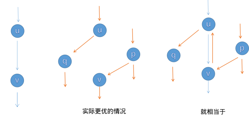
The above example tells us that the "cancellation" effect brought by the push-back operation means we don't need to worry about choosing augmenting paths in the "wrong" order.

It is easy to see that as long as there exists an augmenting path in \(G_f\), augmenting it will increase the total flow; otherwise, it means the total flow has reached its maximum possible value, and the solving process is complete. This is the process of Ford–Fulkerson augmentation.

Max-Flow Min-Cut Theorem

We have a rough understanding of the idea behind Ford–Fulkerson augmentation, but how do we prove the correctness of this method? Why is the flow \(f\) after augmentation completion a maximum flow?

Actually, the correctness of Ford–Fulkerson augmentation is equivalent to the Max-Flow Min-Cut Theorem. This theorem states that for any network \(G = (V, E)\), its maximum flow \(f\) and minimum cut \(\{S, T\}\) always satisfy \(|f| = ||S, T||\).

To prove the Max-Flow Min-Cut Theorem, we start with a lemma: For a network \(G = (V, E)\), take any flow \(f\) and any cut \(\{S, T\}\). We always have \(|f| \leq ||S, T||\), where equality holds if and only if all edges in \(\{(u, v) | u \in S, v \in T\}\) are saturated, and all edges in \(\{(u, v) | u \in T, v \in S\}\) have zero flow.

Proof

\[ \begin{aligned} |f| & = f(s) \\ & = \sum_{u \in S} f(u) \\ & = \sum_{u \in S} \left( \sum_{v \in V} f(u, v) - \sum_{v \in V} f(v, u) \right) \\ & = \sum_{u \in S} \left( \sum_{v \in T} f(u, v) + \sum_{v \in S} f(u, v) - \sum_{v \in T} f(v, u) - \sum_{v \in S} f(v, u) \right) \\ & = \sum_{u \in S} \left( \sum_{v \in T} f(u, v) - \sum_{v \in T} f(v, u) \right) + \sum_{u \in S} \sum_{v \in S} f(u, v) - \sum_{u \in S} \sum_{v \in S} f(v, u) \\ & = \sum_{u \in S} \left( \sum_{v \in T} f(u, v) - \sum_{v \in T} f(v, u) \right) \\ & \leq \sum_{u \in S} \sum_{v \in T} f(u, v) \\ & \leq \sum_{u \in S} \sum_{v \in T} c(u, v) \\ & = ||S, T|| \\ \end{aligned} \]

To achieve equality, the first inequality requires all edges in \(\{(u, v) \mid u \in T, v \in S\}\) to have zero flow, and the second inequality requires all edges in \(\{(u, v) \mid u \in S, v \in T\}\) to be saturated. The lemma is proved.

Now, for any network, can the above equality conditions always be satisfied? If the answer is yes, then the Max-Flow Min-Cut Theorem is proved. Below we attempt to prove this.

Proof

Assume that after a round of augmentation, we obtain a flow \(f\) such that there is no augmenting path in \(G_f\), i.e., there is no path from \(s\) to \(t\) in \(G_f\). At this time, we denote the set of nodes reachable from \(s\) as \(S\), and let \(T = V \setminus S\).

Clearly, \(\{S, T\}\) is a cut in \(G_f\), and \(||S, T|| = \sum_{u \in S} \sum_{v \in T} c_f(u, v) = 0\). Since residual capacities are non-negative, this also means that for any \(u \in S, v \in T, (u, v) \in E_f\), we have \(c_f(u, v) = 0\). Below we discuss these edges in two cases: edges existing in the original graph and reverse edges:

\((u, v) \in E\): In this case, \(c_f(u, v) = c(u, v) - f(u, v) = 0\), so \(c(u, v) = f(u, v)\), i.e., all edges in \(\{(u, v) \mid u \in S, v \in T\}\) are saturated;
\((v, u) \in E\): In this case, \(c_f(u, v) = c(u, v) - f(u, v) = 0 - f(u, v) = f(v, u) = 0\), i.e., all edges in \(\{(v, u) \mid u \in S, v \in T\}\) have zero flow.

Therefore, after augmentation stops, the above flow \(f\) satisfies the equality conditions. According to the size relationship indicated by the lemma, naturally, \(f\) is a maximum flow of \(G\), and \(\{S, T\}\) is a minimum cut of \(G\).

It is easy to see that Kőnig's theorem is a special case of the Max-Flow Min-Cut Theorem. In fact, both are related to duality in linear programming.

Time Complexity Analysis

On a network \(G = (V, E)\) with integer flows, trivially, we assume the flow augmented each time is an integer. Then an upper bound on the time complexity of Ford–Fulkerson augmentation is \(O(|E||f|)\), where \(f\) is the maximum flow on \(G\). This is because the time complexity of a single augmentation round is \(O(|E|)\), and augmentation increases the total flow, so the number of augmentation rounds cannot exceed \(|f|\).

For different implementations of Ford–Fulkerson augmentation, the time complexity varies. Among the mainstream implementations are Edmonds–Karp, Dinic, SAP, ISAP, etc., which we will introduce below.

Edmonds–Karp Algorithm

Algorithm Idea

How to find an augmenting path in \(G_f\)? When considering the specific implementation of Ford–Fulkerson augmentation, the most natural approach is to use BFS. At this point, Ford–Fulkerson augmentation manifests as the Edmonds–Karp algorithm. Its specific steps are as follows:

If we can BFS from \(s\) to \(t\) in \(G_f\), then we have found a new augmenting path.
For the augmenting path \(p\), we compute the minimum residual capacity along the path: \(\Delta = \min_{(u, v) \in p} c_f(u, v)\). We add \(\Delta\) flow to each edge on \(p\) and push back \(\Delta\) flow on their reverse edges, increasing the maximum flow by \(\Delta\).
Because we modified the flow, we obtain a new \(G_f\). We repeat the above process on the new \(G_f\) until no augmenting path exists, meaning the flow no longer increases.

The above algorithm is the Edmonds–Karp algorithm.

Time Complexity Analysis

Next, let's try to analyze the time complexity of the Edmonds–Karp algorithm.

Clearly, the time complexity of a single BFS augmentation round is \(O(|E|)\).

The upper bound on the total number of augmentation rounds is \(O(|V||E|)\). This claim is often falsely proven (or glossed over) in online materials. Below we attempt to provide a more formal proof¹.

Proof of Upper Bound on Total Augmentation Rounds

First, we introduce a lemma—the non-decreasing shortest path lemma. Specifically, we denote \(d_f(u)\) as the distance (i.e., shortest path length) from node \(u\) to source \(s\) in \(G_f\). For a given augmentation round, let \(f\) and \(f'\) denote the flow before and after augmentation, respectively. We assert that for any node \(u\), augmentation always ensures \(d_{f'}(u) \geq d_f(u)\). We will prove this lemma shortly.

Let the edge with the smallest residual capacity on the augmenting path be called a saturated edge (if multiple edges tie for the minimum, pick any). If a directed edge \((u, v)\) is chosen as a saturated edge, augmentation will clear its residual capacity, causing the saturated edge to disappear, and push-back will create a new reverse edge (if it didn't exist before), i.e., \((u, v) \not \in E_{f'}\) and \((v, u) \in E_{f'}\). The above analysis tells us that for an undirected edge \((u, v)\), the two directions in which it is augmented always alternate.

When augmenting along \((u, v)\) in \(G_f\), \(d_f(u) + 1 = d_f(v)\). Afterward, the residual network becomes \(G_{f'}\). When augmenting along \((v, u)\) in \(G_{f'}\), \(d_{f'}(v) + 1 = d_{f'}(u)\). According to the non-decreasing shortest path lemma, we also have \(d_{f'}(v) \geq d_f(v)\). Combining all equations, we get \(d_{f'}(u) \geq d_{f}(u) + 2\). In other words, if directed edge \((u, v)\) is chosen as a saturated edge, then compared to the last time it was chosen as a saturated edge, the distance from \(u\) to \(s\) increases by at least \(2\).

The distance from \(s\) to any node cannot exceed \(|V|\). Combining this with the above property, we find that each edge is chosen as a saturated edge \(O(|V|)\) times. Multiplying by the number of edges gives an upper bound of \(O(|V||E|)\) on the total number of augmentation rounds.

Next, we prove the non-decreasing shortest path lemma, i.e., \(d_{f'}(u) \geq d_f(u)\). This proof is not difficult but may be slightly convoluted; readers can pause and think carefully.

Proof of Non-Decreasing Shortest Path Lemma

Assume for contradiction. For a certain augmentation round, suppose there exist nodes whose distance to \(s\) decreases after augmentation compared to before. Let \(v\) be the one with the smallest distance to \(s\) after augmentation (i.e., \(v = \arg \min_{x \in V, d_{f'}(x) < d_f(x)} d_{f'}(x)\)). Note, by the assumption of contradiction, \(d_{f'}(v) < d_f(v)\) is known.

On the shortest path from \(s\) to \(v\) in \(G_{f'}\), let \(u\) be the node preceding \(v\), i.e., \(d_{f'}(u) + 1 = d_{f'}(v)\).

To prevent \(u\) from violating the "minimum distance" property of \(v\), \(u\) must satisfy \(d_{f'}(u) \geq d_f(u)\).

Adding \(1\) to both sides of the inequality, we get \(d_{f'}(v) \geq d_f(u) + 1\). Using the contradiction assumption to relax, we get \(d_f(v) > d_f(u) + 1\).

Below we try to discuss the direction of augmentation on \((u, v)\).

Suppose directed edge \((u, v) \in E_f\). By the "breadth-first" property of BFS, we have \(d_f(u) + 1 \geq d_f(v)\). This conflicts with the relaxed result, leading to a contradiction.
Suppose directed edge \((u, v) \not \in E_f\). By the definition of \(u\), we know \((u, v) \in E_{f'}\). Therefore, the existence of this edge must be the result of the current augmentation round passing through \((v, u)\) and pushing back to create a reverse edge, i.e., \(d_f(v) + 1 = d_f(u)\). This conflicts with the relaxed result, leading to a contradiction.

Since augmenting \((u, v)\) in any direction leads to a contradiction, we know the assumption is false, and the non-decreasing shortest path lemma is proved.

Multiplying the complexity of a single BFS augmentation round by the upper bound on the number of augmentation rounds, we get that the time complexity of the Edmonds–Karp algorithm is \(O(|V||E|^2)\).

Code Implementation

A possible implementation of the Edmonds–Karp algorithm is as follows.

Reference Code

constexpr int MAXN = 250;
constexpr int INF = 0x3f3f3f3f;

struct Edge {
  int from, to, cap, flow;

  Edge(int u, int v, int c, int f) : from(u), to(v), cap(c), flow(f) {}
};

struct EK {
  int n, m;             // n: number of nodes, m: number of edges
  vector<Edge> edges;   // edges: collection of all edges
  vector<int> G[MAXN];  // G: node x -> indices of all edges from x in edges
  int a[MAXN], p[MAXN]; // a: node x -> maximum flow assigned to it by the edge closest to x during BFS
                        // p: node x -> edge closest to x during BFS

  void init(int n) {
    for (int i = 0; i < n; i++) G[i].clear();
    edges.clear();
  }

  void AddEdge(int from, int to, int cap) {
    edges.push_back(Edge(from, to, cap, 0));
    edges.push_back(Edge(to, from, 0, 0));
    m = edges.size();
    G[from].push_back(m - 2);
    G[to].push_back(m - 1);
  }

  int Maxflow(int s, int t) {
    int flow = 0;
    for (;;) {
      memset(a, 0, sizeof(a));
      queue<int> Q;
      Q.push(s);
      a[s] = INF;
      while (!Q.empty()) {
        int x = Q.front();
        Q.pop();
        for (int i = 0; i < G[x].size(); i++) {  // iterate over edges starting from x
          Edge& e = edges[G[x][i]];
          if (!a[e.to] && e.cap > e.flow) {
            p[e.to] = G[x][i];  // G[x][i] is the edge closest to node e.to
            a[e.to] =
                min(a[x], e.cap - e.flow);  // assign flow to node e.to from the closest edge
            Q.push(e.to);
          }
        }
        if (a[t]) break;  // if the sink receives flow, exit BFS
      }
      if (!a[t])
        break;  // if the sink does not receive flow, source and sink are not in the same connected component
      for (int u = t; u != s;
           u = edges[p[u]].from) {  // trace the path s -> t during BFS via u
        edges[p[u]].flow += a[t];      // increase flow on edges along the path
        edges[p[u] ^ 1].flow -= a[t];  // decrease flow on reverse edges
      }
      flow += a[t];
    }
    return flow;
  }
};

Dinic Algorithm

Algorithm Idea

Consider performing BFS layering on \(G_f\) before augmentation, i.e., dividing nodes into layers based on their distance \(d(u)\) from source \(s\). Allow flow passing through \(u\) to only go to nodes \(v\) in the next layer, i.e., remove outgoing edges from \(u\) to nodes with the same or smaller layer numbers. We call the remaining part of \(G_f\) the level graph (Level Graph). Formally, we say \(G_L = (V, E_L)\) is the level graph of \(G_f = (V, E_f)\), where \(E_L = \left\{ (u, v) \mid (u, v) \in E_f, d(u) + 1 = d(v) \right\}\).

If we find a maximal augmenting flow \(f_b\) on the level graph \(G_L\) such that it is impossible to further increase \(f_b\) on \(G_L\) alone, we call \(f_b\) a blocking flow (Blocking Flow) of \(G_L\).

Warning

Although we defined augmentation/augmenting flow only on a single augmenting path above, broadly, the term "augmentation" can refer not only to augmenting flow on a single path but also to the union of several augmenting flows—the latter is the meaning used when defining blocking flow.

After defining level graph and blocking flow, the Dinic algorithm proceeds as follows.

Perform BFS on \(G_f\) to obtain the level graph \(G_L\).
Perform DFS on \(G_L\) to find a blocking flow \(f_b\).
Merge \(f_b\) into the original flow \(f\), i.e., \(f \leftarrow f + f_b\).
Repeat the above process until there is no path from \(s\) to \(t\).

At this point, \(f\) is the maximum flow.

Before analyzing the complexity of this algorithm, we need to specifically explain the process of "performing DFS on \(G_L\) to find a blocking flow \(f_b\)". While BFS for the level graph should be trivial for readers of this page, the process of DFS for blocking flow requires some technique—we need to introduce the current arc optimization.

Note that during DFS on \(G_L\), if a node \(u\) has many incoming and outgoing edges, and each time \(u\) receives flow from incoming edges, it iterates over its outgoing edge list to decide which outgoing edge to pass the flow to, then the worst-case local time complexity for \(u\) could be \(O(|E|^2)\). To avoid this defect, if at some point we know that edge \((u, v)\) has been augmented to its limit (edge \((u, v)\) has no remaining capacity or \(v\)'s downstream is already blocked), then \(u\)'s flow need not attempt to go to outgoing edge \((u, v)\). Accordingly, for each node \(u\), we maintain the first outgoing edge from \(u\)'s list that is still worth trying. Conventionally, we call this maintained pointer the current arc, and this approach current arc optimization.

Multi-way Augmentation

Multi-way augmentation is a constant optimization for the Dinic algorithm—if we find an augmenting path \(p\) from \(s\) to \(t\) on the level graph, we may not need to restart from \(s\) to find the next augmenting path; instead, we can start from the last position on \(p\) that still has residual capacity to find a branching path for augmentation. Considering its consistency with the backtracking form, this optimization is also natural in the DFS code implementation.

Common Misconception

Possibly due to erroneous descriptions in many online materials leading to misinformation, a considerable number of contestants like to list current arc optimization and multi-way augmentation as two separate optimizations of the Dinic algorithm. Actually, current arc optimization is part of ensuring the correctness of Dinic's time complexity, while multi-way augmentation is merely a constant optimization that does not affect complexity.

Time Complexity Analysis

After applying current arc optimization, the time complexity analysis of the Dinic algorithm is as follows.

First, we try to prove that the time complexity of DFS for finding a blocking flow in a single augmentation round is \(O(|V||E|)\).

Proof of Time Complexity for Single Augmentation Round

Consider each augmenting path in the blocking flow \(f_b\). They are all obtained by jumping along current arcs in \(G_L\), and each augmenting path cannot experience more than \(|V|\) jumps.

Each time an augmenting path is found, a saturated edge disappears (residual capacity becomes zero). Consider each augmenting path in the blocking flow \(f_b\). Denote the set of saturated edges cleared by them as \(E_1\). Considering the layering property of \(G_L\), after a saturated edge disappears, its reverse edge cannot be traversed by other augmenting paths in the same augmentation round. Therefore, \(E_1\) is a subset of \(E_L\).

Additionally, for cases where we jump along the current arc but fail to obtain a complete augmenting path due to blocking at some position, we denote the set of last edges on these incomplete paths as \(E_2\). Members of \(E_2\) are not saturated, so \(E_1\) and \(E_2\) are disjoint, and \(E_1 \cup E_2\) is still a subset of \(E_L\).

Since each member of \(E_1 \cup E_2\) does not incur more than \(|V|\) jumps (and with multi-way augmentation optimization, some jumps may be counted multiple times), in summary, the total number of jumps during DFS cannot exceed \(|V||E_L|\).

A Common False Proof

For each node, we maintain the next edge that can be augmented, and the current arc changes at most \(|E|\) times, so the worst-case time complexity of a single augmentation round is \(O(|V||E|)\).

Bug

"The current arc changes at most \(|E|\) times" does not imply "each node visits its outgoing edges at most \(|E|\) times." This is because visiting the current arc does not necessarily exhaust its residual capacity; node \(u\) may visit the same current arc multiple times.

Note that the number of layers in the level graph obviously cannot exceed \(|V|\). If we can prove that the number of layers strictly increases during augmentation, then the number of augmentation rounds in Dinic's algorithm is \(O(|V|)\). Next, we try to prove this claim².

Proof of Monotonicity of Level Graph Layers

We need to introduce a concept from preflow-push algorithms (another class of maximum flow algorithms)—height labels. To more conveniently combine height labels in our proof, during the proof, we let \(d_f(u)\) be the distance from node \(u\) to the sink \(t\) in \(G_f\), layering from the sink rather than the source (this makes no essential difference). For a given augmentation round, let \(f\) and \(f'\) denote the flow before and after augmentation, respectively. After solving and adding the blocking flow in this round, denote the level graph changing from \(G_L = (V, E_L)\) to \(G'_{L} = (V, E'_L)\).

We give a non-strict temporary definition of height labels—on a network \(G = (V, E)\), let \(h\) be a function from node set \(V\) to the set of integers \(N\). \(h\) is a valid height label on \(G\) if and only if \(h(u) \leq h(v) + 1\) holds for all \((u, v) \in E\).

Examining all members \((u, v)\) of \(E_{f'}\), we find that \((u, v) \in E_{f'}\) for one of two reasons:

\((u, v) \in E_f\), and the residual capacity was not exhausted during this augmentation round—by the definition of shortest path, we have \(d_f(u) \leq d_f(v) + 1\);
\((u, v) \not \in E_f\), but during this augmentation round, the blocking flow passed through \((v, u)\) and pushed back, creating a reverse edge—by the definitions of level graph and blocking flow, we have \(d_f(u) + 1 = d_f(v)\).

The above observation leads us to a conclusion—\(d_f\) is a valid height label on \(G_{f'}\). Of course, it is also valid on \(G'_L\), a subgraph of \(G_{f'}\).

Now, for an augmenting path \(p = (s, \dots, u, v, \dots, t)\) on \(G'_L\), consider the process of adding nodes one by one in reverse order (from \(t\) to \(s\)) starting from an empty path. Suppose node \(v\) has been added, and node \(u\) is being added. We find that after adding node \(u\), by the definition of the level graph, the value of \(d_{f'}(u)\) increases by \(1\) compared to \(d_{f'}(v)\); meanwhile, since \(d_f\) is a height label on \(G'_L\), the value of \(d_f(u)\) may increase by \(1\), remain unchanged, or decrease compared to \(d_f(v)\). Therefore, after the entire path is added, we get \(d_{f'}(s) \geq d_f(s)\), where equality holds if and only if \(d_f(u) = d_f(v) + 1\) for all \((u, v) \in p\). If this inequality cannot hold with equality, then \(d_{f'}(s) > d_f(s)\)—which is the desired conclusion "the number of layers in the level graph strictly increases during augmentation." Below we try to prove that the inequality cannot hold with equality.

Assume for contradiction that \(d_{f'}(s) = d_f(s)\) holds, and try to derive a contradiction. Now we assert that on \(G'_L\), \(p\) contains at least one edge \((u, v)\) such that \((u, v)\) does not exist in \(G_L\). If there is no such edge, considering \(d_f(s) = d_{f'}(s)\) and the definitions of level graph and blocking flow, augmentation on \(G_L\) should not have completed yet. To avoid this contradiction, our assertion must be true.

Let \((u, v)\) be that edge satisfying the assertion condition. The reason it satisfies the assertion can only be one of the following:

\((u, v) \in E_f\) but \(d_f(u) \leq d_f(v) + 1\) does not hold with equality, so by the definition of the level graph, \((u, v) \not \in E_L\), and it is added to \(E'_L\) during the new layering after augmentation;
\((u, v) \not \in E_f\), meaning the creation of edge \((u, v)\) is the result of the blocking flow passing through \((v, u)\) and pushing back to create a reverse edge in the current augmentation round, i.e., \(d_f(u) = d_f(v) - 1\).

Since in either way of satisfying the assertion we get \(d_f(u) \neq d_f(v) + 1\), i.e., the condition for equality \(d_{f'}(s) \geq d_f(s)\) cannot be satisfied, this conflicts with the assumption \(d_{f'}(s) = d_f(s)\). The original proposition is proved.

Another Common False Proof

Assume for contradiction. Suppose the number of layers in the level graph remains the same after an augmentation round. Then there should still be at least one augmenting path from \(s\) to \(t\) on the level graph where the layer difference between adjacent nodes is \(1\). The fact that this augmenting path was not augmented means the augmentation round has not finished. To avoid the above contradiction, the original proposition holds.

Bug

"The new level graph after an augmentation round has the same \(s\)-\(t\) shortest distance as before" does not imply "the augmentation round on the old level graph has not finished." This is because there is no reason to assume the edge sets of the two level graphs are the same; the \(s\)-\(t\) shortest path on the new level graph might pass through edges not present in the old level graph.

Multiplying the time complexity of a single augmentation round \(O(|V||E|)\) by the number of augmentation rounds \(O(|V|)\), the time complexity of the Dinic algorithm is \(O(|V|^2|E|)\).

If we want the actual running time of Dinic's algorithm to approach its theoretical upper bound, we need to construct networks with special properties as input. In algorithm competition practice, assessments related to network flow knowledge often focus on the skill of modeling the original problem as a network flow problem. At this time, our modeling usually does not include special properties that make Dinic's algorithm slow; on the contrary, Dinic's algorithm is very efficient on most graphs. Therefore, the data ranges for network flow problems are usually large, and the method of "substituting \(|V|, |E|\) into \(|V|^2|E|\) to estimate running time" is not applicable. Actually, accurate estimation requires some experience from the contestant regarding the actual efficiency of Dinic's algorithm; readers can practice more.

Time Complexity Analysis in Special Cases

On some well-behaved graphs, Dinic's algorithm has better time complexity.

For a network \(G = (V, E)\), if all edge capacities are \(1\), i.e., \(c(u, v) \in \{0, 1\}\) for all \((u, v) \in E\), we call \(G\) unit capacity.

In unit capacity networks, the time complexity of a single augmentation round in Dinic's algorithm is \(O(|E|)\).

Proof

This is because each augmentation causes all edges on the augmenting path to become saturated and disappear, so each edge can be augmented at most once per augmentation round.

In unit capacity networks, the number of augmentation rounds in Dinic's algorithm is \(O(|E|^{\frac{1}{2}})\).

Proof

Layer with source \(s\) as the center. Denote \(d_f(u)\) as the distance from node \(u\) to source \(s\) in \(G_f\). Additionally, define the set of points \(\left\{u \mid u \in V, d_f(u) = k \right\}\) as layer \(D_k\) with number \(k\), and let \(S_k = \cup_{i \leq k} D_i\).

Suppose we have performed \(|E|^{\frac{1}{2}}\) augmentation rounds. By the pigeonhole principle, there exists at least one \(k\) such that the size of the edge set \(\left\{ (u, v) \mid u \in D_k, v \in D_{k+1}, (u, v) \in E_f \right\}\) is at most \(\frac {|E|} {|E|^{\frac{1}{2}}} \approx |E|^{\frac{1}{2}}\). Clearly, \(\{S_k, V - S_k\}\) is an \(s\)-\(t\) cut on \(G_f\), and its cut capacity does not exceed \(|E|^{\frac{1}{2}}\). By the Max-Flow Min-Cut Theorem, the maximum flow on \(G_f\) does not exceed \(|E|^{\frac{1}{2}}\), i.e., at most \(|E|^{\frac{1}{2}}\) more augmentation rounds can be performed on \(G_f\). Therefore, the total number of augmentation rounds is \(O(|E|^{\frac{1}{2}})\).

In unit capacity networks, the number of augmentation rounds in Dinic's algorithm is \(O(|V|^{\frac{2}{3}})\).

Proof

Suppose we have performed \(2 |V|^{\frac{2}{3}}\) augmentation rounds. Since at most half (\(|V|^{\frac{2}{3}}\)) of the layers contain more than \(|V|^{\frac{1}{3}}\) nodes, no matter how we distribute the sizes of all layers, there exists at least one \(k\) such that two adjacent layers both contain no more than \(|V|^{\frac{1}{3}}\) nodes, i.e., \(|D_k| \leq |V|^{\frac{1}{3}}\) and \(|D_{k+1}| \leq |V|^{\frac{1}{3}}\).

To maximize the number of edges between \(D_k\) and \(D_{k+1}\), assume it is a complete bipartite graph. Then the size of edge set \(\left\{ (u, v) \mid u \in D_k, v \in D_{k+1}, (u, v) \in E_f \right\}\) is at most \(|V|^{\frac{2}{3}}\). Clearly, \(\{S_k, V - S_k\}\) is an \(s\)-\(t\) cut on \(G_f\), and its cut capacity does not exceed \(|V|^{\frac{2}{3}}\). By the Max-Flow Min-Cut Theorem, the maximum flow on \(G_f\) does not exceed \(|V|^{\frac{2}{3}}\), i.e., at most \(|V|^{\frac{2}{3}}\) more augmentation rounds can be performed on \(G_f\). Therefore, the total number of augmentation rounds is \(O(|V|^{\frac{2}{3}})\).

In unit capacity networks, if every node \(u\) other than source and sink satisfies \(\mathit{deg}_{\mathit{in}}(u) = 1\) or \(\mathit{deg}_{\mathit{out}}(u) = 1\), then the number of augmentation rounds in Dinic's algorithm is \(O(|V|^{\frac{1}{2}})\). Here, \(\mathit{deg}_{\mathit{in}}(u)\) and \(\mathit{deg}_{\mathit{out}}(u)\) represent the in-degree and out-degree of node \(u\), respectively.

Proof

We introduce the following lemma—for networks of this form, any flow on them can always be decomposed into several unit-flow augmenting paths that are vertex-disjoint.

Suppose we have performed \(|V|^{\frac{1}{2}}\) augmentation rounds. By the definition of the level graph, any new augmenting path now has length at least \(|V|^{\frac{1}{2}}\).

Consider the augmenting path decomposition of the maximum flow on \(G_f\). The number of augmenting paths we obtain cannot exceed \(\frac {|V|} {|V|^{\frac{1}{2}}} \approx |V|^{\frac{1}{2}}\), meaning at most \(|V|^{\frac{1}{2}}\) more augmentation rounds can be performed on \(G_f\). Therefore, the total number of augmentation rounds is \(O(|V|^{\frac{1}{2}})\).

In summary, we derive some corollaries.

On unit capacity networks, the total time complexity of Dinic's algorithm is \(O(|E| \min(|E|^\frac{1}{2}, |V|^{\frac{2}{3}}))\).
On unit capacity networks, if every node \(u\) other than source and sink satisfies \(\mathit{deg}_{\mathit{in}}(u) = 1\) or \(\mathit{deg}_{\mathit{out}}(u) = 1\), the total time complexity of Dinic's algorithm is \(O(|E||V|^{\frac{1}{2}})\). For the bipartite maximum matching problem, we often use the Hopcroft–Karp algorithm, which is actually a special case of Dinic's algorithm on unit capacity networks satisfying the above degree restrictions.

Code Implementation

Reference Code

struct MF {
  struct edge {
    int v, nxt, cap, flow;
  } e[N];

  int fir[N], cnt = 0;

  int n, S, T;
  ll maxflow = 0;
  int dep[N], cur[N];

  void init() {
    memset(fir, -1, sizeof fir);
    cnt = 0;
  }

  void addedge(int u, int v, int w) {
    e[cnt] = {v, fir[u], w, 0};
    fir[u] = cnt++;
    e[cnt] = {u, fir[v], 0, 0};
    fir[v] = cnt++;
  }

  bool bfs() {
    queue<int> q;
    memset(dep, 0, sizeof(int) * (n + 1));

    dep[S] = 1;
    q.push(S);
    while (q.size()) {
      int u = q.front();
      q.pop();
      for (int i = fir[u]; ~i; i = e[i].nxt) {
        int v = e[i].v;
        if ((!dep[v]) && (e[i].cap > e[i].flow)) {
          dep[v] = dep[u] + 1;
          q.push(v);
        }
      }
    }
    return dep[T];
  }

  int dfs(int u, int flow) {
    if ((u == T) || (!flow)) return flow;

    int ret = 0;
    for (int& i = cur[u]; ~i; i = e[i].nxt) {
      int v = e[i].v, d;
      if ((dep[v] == dep[u] + 1) &&
          (d = dfs(v, min(flow - ret, e[i].cap - e[i].flow)))) {
        ret += d;
        e[i].flow += d;
        e[i ^ 1].flow -= d;
        if (ret == flow) return ret;
      }
    }
    return ret;
  }

  void dinic() {
    while (bfs()) {
      memcpy(cur, fir, sizeof(int) * (n + 1));
      maxflow += dfs(S, INF);
    }
  }
} mf;

MPM Algorithm

MPM (Malhotra, Pramodh-Kumar and Maheshwari) algorithm obtains the maximum flow in two ways: using a heap-based priority queue with time complexity \(O(n^3\log n)\); commonly using a BFS solution with time complexity \(O(n^3)\). Note, this section focuses only on analyzing the better and more concise \(O(n^3)\) algorithm.

The overall structure of the MPM algorithm is similar to Dinic's algorithm, also running in phases. In each phase, find augmenting paths in the layered network of the residual network of \(G\). The main difference from Dinic's algorithm lies in the way augmenting paths are found: the part of MPM that finds augmenting paths takes only \(O(n^2)\), which is better than Dinic's algorithm in time complexity.

The MPM algorithm considers vertex capacities rather than edge capacities. In the layered network \(L\), if we define the capacity \(p(v)\) of a vertex \(v\) as the minimum of its incoming residual and outgoing residual, then:

\[ \begin{aligned} p_{in}(v) &= \sum\limits_{(u,v) \in L} (c(u, v) - f(u, v)) \\ p_{out}(v) &= \sum\limits_{(v,u) \in L} (c(v, u) - f(v, u)) \\ p(v) &= \min (p_{in}(v), p_{out}(v)) \end{aligned} \]

We call a node \(r\) a reference node if and only if \(p(r) = \min {p(v)}\). For a reference node \(r\), we can always increase the flow passing through \(r\) by \(p(r)\) to make its capacity \(0\). This is because \(L\) is a directed acyclic graph and node capacities in \(L\) are at least \(p(r)\), so we can always find a directed path from \(s\) through \(r\) to \(t\). Then we increase the flow on all edges along this path by \(p(r)\). This path is the augmenting path for this phase. Finding augmenting paths can be done with BFS. After augmentation, all saturated edges can be removed from \(L\) because they will not be used after this phase. Similarly, all nodes other than \(s\) and \(t\) that have no outgoing or incoming edges can be deleted.

Time Complexity Analysis

Each phase of the MPM algorithm requires \(O(V^2)\), because there are at most \(V\) iterations (since at least the selected reference node is deleted), and in each iteration, we delete all edges passing through except at most \(V\). Summing, we get \(O(V^2+E)=O(V^2)\). Since the total number of phases is less than \(V\), the total running time of the MPM algorithm is \(O(V^3)\).

Proof that Total Number of Phases is Less Than V

The MPM algorithm terminates in fewer than \(V\) phases. To prove this, we must first prove two lemmas.

Lemma 1: After each iteration, the distance from \(s\) to each point does not decrease, i.e., \(level_{i+1}[v] \ge level_{i}[v]\).

Proof: Fix a phase \(i\) and a point \(v\). Consider any shortest path \(P\) from \(s\) to \(v\) in \(G_{i}^R\). The length of \(P\) equals \(level_{i}[v]\). Note \(G_{i}^R\) can only contain backward edges and forward edges of \(G_{i}^R\). If \(P\) has no backward edges of \(G_{i}^R\), then \(level_{i+1}[v] \ge level_{i}[v]\) because \(P\) is also a path in \(G_{i}^R\). Now, suppose \(P\) has at least one backward edge and the first such edge is \((u,w)\). Then \(level_{i+1}[u] \ge level_{i}[u]\) (because of the first case). Edge \((u,w)\) does not belong to \(G_{i}^R\), so \((u,w)\) is affected by the augmenting path of the previous iteration. This means \(level_{i}[u] = level_{i}[w]+1\). Also, \(level_{i+1}[w] = level_{i+1}[u]+1\). From these two equations and \(level_{i+1}[u] \ge level_{i}[u]\), we get \(level_{i+1}[w] \ge level_{i}[w]+2\). The rest of the path can be handled similarly.

Lemma 2: \(level_{i+1}[t] > level_{i}[t]\).

Proof: From Lemma 1 we have \(level_{i+1}[t] \ge level_{i}[t]\). Suppose \(level_{i+1}[t] = level_{i}[t]\). Note \(G_{i}^R\) can only contain backward edges and forward edges of \(G_{i}^R\). This means there is a shortest path in \(G_{i}^R\) not blocked by augmenting paths. This is a contradiction.

Implementation

Reference Code

struct MPM {
  struct FlowEdge {
    int v, u;
    long long cap, flow;

    FlowEdge() {}

    FlowEdge(int _v, int _u, long long _cap, long long _flow)
        : v(_v), u(_u), cap(_cap), flow(_flow) {}

    FlowEdge(int _v, int _u, long long _cap)
        : v(_v), u(_u), cap(_cap), flow(0ll) {}
  };

  constexpr static long long flow_inf = 1e18;
  vector<FlowEdge> edges;
  vector<char> alive;
  vector<long long> pin, pout;
  vector<list<int>> in, out;
  vector<vector<int>> adj;
  vector<long long> ex;
  int n, m = 0;
  int s, t;
  vector<int> level;
  vector<int> q;
  int qh, qt;

  void resize(int _n) {
    n = _n;
    ex.resize(n);
    q.resize(n);
    pin.resize(n);
    pout.resize(n);
    adj.resize(n);
    level.resize(n);
    in.resize(n);
    out.resize(n);
  }

  MPM() {}

  MPM(int _n, int _s, int _t) {
    resize(_n);
    s = _s;
    t = _t;
  }

  void add_edge(int v, int u, long long cap) {
    edges.push_back(FlowEdge(v, u, cap));
    edges.push_back(FlowEdge(u, v, 0));
    adj[v].push_back(m);
    adj[u].push_back(m + 1);
    m += 2;
  }

  bool bfs() {
    while (qh < qt) {
      int v = q[qh++];
      for (int id : adj[v]) {
        if (edges[id].cap - edges[id].flow < 1) continue;
        if (level[edges[id].u] != -1) continue;
        level[edges[id].u] = level[v] + 1;
        q[qt++] = edges[id].u;
      }
    }
    return level[t] != -1;
  }

  long long pot(int v) { return min(pin[v], pout[v]); }

  void remove_node(int v) {
    for (int i : in[v]) {
      int u = edges[i].v;
      auto it = find(out[u].begin(), out[u].end(), i);
      out[u].erase(it);
      pout[u] -= edges[i].cap - edges[i].flow;
    }
    for (int i : out[v]) {
      int u = edges[i].u;
      auto it = find(in[u].begin(), in[u].end(), i);
      in[u].erase(it);
      pin[u] -= edges[i].cap - edges[i].flow;
    }
  }

  void push(int from, int to, long long f, bool forw) {
    qh = qt = 0;
    ex.assign(n, 0);
    ex[from] = f;
    q[qt++] = from;
    while (qh < qt) {
      int v = q[qh++];
      if (v == to) break;
      long long must = ex[v];
      auto it = forw ? out[v].begin() : in[v].begin();
      while (true) {
        int u = forw ? edges[*it].u : edges[*it].v;
        long long pushed = min(must, edges[*it].cap - edges[*it].flow);
        if (pushed == 0) break;
        if (forw) {
          pout[v] -= pushed;
          pin[u] -= pushed;
        } else {
          pin[v] -= pushed;
          pout[u] -= pushed;
        }
        if (ex[u] == 0) q[qt++] = u;
        ex[u] += pushed;
        edges[*it].flow += pushed;
        edges[(*it) ^ 1].flow -= pushed;
        must -= pushed;
        if (edges[*it].cap - edges[*it].flow == 0) {
          auto jt = it;
          ++jt;
          if (forw) {
            in[u].erase(find(in[u].begin(), in[u].end(), *it));
            out[v].erase(it);
          } else {
            out[u].erase(find(out[u].begin(), out[u].end(), *it));
            in[v].erase(it);
          }
          it = jt;
        } else
          break;
        if (!must) break;
      }
    }
  }

  long long flow() {
    long long ans = 0;
    while (true) {
      pin.assign(n, 0);
      pout.assign(n, 0);
      level.assign(n, -1);
      alive.assign(n, true);
      level[s] = 0;
      qh = 0;
      qt = 1;
      q[0] = s;
      if (!bfs()) break;
      for (int i = 0; i < n; i++) {
        out[i].clear();
        in[i].clear();
      }
      for (int i = 0; i < m; i++) {
        if (edges[i].cap - edges[i].flow == 0) continue;
        int v = edges[i].v, u = edges[i].u;
        if (level[v] + 1 == level[u] && (level[u] < level[t] || u == t)) {
          in[u].push_back(i);
          out[v].push_back(i);
          pin[u] += edges[i].cap - edges[i].flow;
          pout[v] += edges[i].cap - edges[i].flow;
        }
      }
      pin[s] = pout[t] = flow_inf;
      while (true) {
        int v = -1;
        for (int i = 0; i < n; i++) {
          if (!alive[i]) continue;
          if (v == -1 || pot(i) < pot(v)) v = i;
        }
        if (v == -1) break;
        if (pot(v) == 0) {
          alive[v] = false;
          remove_node(v);
          continue;
        }
        long long f = pot(v);
        ans += f;
        push(v, s, f, false);
        push(v, t, f, true);
        alive[v] = false;
        remove_node(v);
      }
    }
    return ans;
  }
};

ISAP

In Dinic's algorithm, we run BFS to layer after each augmentation. Is there a more efficient method?

The answer is the ISAP algorithm introduced below.

Process

Like Dinic's algorithm, we first run BFS to layer the nodes on the graph. However, slightly different from Dinic, we choose to perform BFS from the sink \(t\) to the source \(s\) on the reverse graph.

After the layering process, we use DFS to find augmenting paths.

The augmentation process is similar to Dinic: we only choose nodes whose layer is exactly \(1\) less than the current node for augmentation.

Unlike Dinic, we do not rerun BFS to relayer the nodes on the graph; instead, the relabeling process is completed during augmentation.

Specifically, let the layer of node \(i\) be \(d_i\). When we finish augmenting at node \(i\), we traverse all outgoing edges of \(i\) in the residual network, find the outgoing node \(j\) with the smallest layer, and then set \(d_i \gets d_j+1\). In particular, if \(i\) has no outgoing edges in the residual network, then \(d_i \gets n\).

It is easy to see that when \(d_s \geq n\), there is no augmenting path in the graph, and the algorithm can terminate.

Like Dinic, ISAP also has current arc optimization.

ISAP also has another optimization: we record the number of nodes at layer \(i\) as \(num_i\). Whenever a node's layer is updated from \(x\) to \(y\), we simultaneously update the \(num\) array. If after updating, \(num_x=0\), it means a gap has appeared in the graph, and no augmenting path can be found. At this point, we can directly terminate the algorithm (in implementation, simply mark \(d_s\) as \(n\)). This optimization is called GAP optimization.

Implementation

Reference Code

struct Edge {
  int from, to, cap, flow;

  Edge(int u, int v, int c, int f) : from(u), to(v), cap(c), flow(f) {}
};

bool operator<(const Edge& a, const Edge& b) {
  return a.from < b.from || (a.from == b.from && a.to < b.to);
}

struct ISAP {
  int n, m, s, t;
  vector<Edge> edges;
  vector<int> G[MAXN];
  bool vis[MAXN];
  int d[MAXN];
  int cur[MAXN];
  int p[MAXN];
  int num[MAXN];

  void AddEdge(int from, int to, int cap) {
    edges.push_back(Edge(from, to, cap, 0));
    edges.push_back(Edge(to, from, 0, 0));
    m = edges.size();
    G[from].push_back(m - 2);
    G[to].push_back(m - 1);
  }

  bool BFS() {
    memset(vis, 0, sizeof(vis));
    queue<int> Q;
    Q.push(t);
    vis[t] = true;
    d[t] = 0;
    while (!Q.empty()) {
      int x = Q.front();
      Q.pop();
      for (int i = 0; i < G[x].size(); i++) {
        Edge& e = edges[G[x][i] ^ 1];
        if (!vis[e.from] && e.cap > e.flow) {
          vis[e.from] = true;
          d[e.from] = d[x] + 1;
          Q.push(e.from);
        }
      }
    }
    return vis[s];
  }

  void init(int n) {
    this->n = n;
    for (int i = 0; i < n; i++) G[i].clear();
    edges.clear();
  }

  int Augment() {
    int x = t, a = INF;
    while (x != s) {
      Edge& e = edges[p[x]];
      a = min(a, e.cap - e.flow);
      x = edges[p[x]].from;
    }
    x = t;
    while (x != s) {
      edges[p[x]].flow += a;
      edges[p[x] ^ 1].flow -= a;
      x = edges[p[x]].from;
    }
    return a;
  }

  int Maxflow(int s, int t) {
    this->s = s;
    this->t = t;
    int flow = 0;
    BFS();
    memset(num, 0, sizeof(num));
    for (int i = 0; i < n; i++) num[d[i]]++;
    int x = s;
    memset(cur, 0, sizeof(cur));
    while (d[s] < n) {
      if (x == t) {
        flow += Augment();
        x = s;
      }
      int ok = 0;
      for (int i = cur[x]; i < G[x].size(); i++) {
        Edge& e = edges[G[x][i]];
        if (e.cap > e.flow && d[x] == d[e.to] + 1) {
          ok = 1;
          p[e.to] = G[x][i];
          cur[x] = i;
          x = e.to;
          break;
        }
      }
      if (!ok) {
        int m = n - 1;
        for (int i = 0; i < G[x].size(); i++) {
          Edge& e = edges[G[x][i]];
          if (e.cap > e.flow) m = min(m, d[e.to]);
        }
        if (--num[d[x]] == 0) break;
        num[d[x] = m + 1]++;
        cur[x] = 0;
        if (x != s) x = edges[p[x]].from;
      }
    }
    return flow;
  }
};

Push-Relabel Preflow-Push Algorithm

This method ignores flow conservation during the solving process and updates information for one node at a time to solve the maximum flow.

Generic Preflow-Push Algorithm

First, we introduce the main idea of the preflow-push algorithm and a feasible brute-force implementation.

The preflow-push algorithm solves the maximum flow by performing update operations on individual nodes until no node needs updating.

The flow function maintained during the algorithm process does not necessarily preserve flow conservation. For a node, we allow the incoming flow to exceed the outgoing flow. The excess part is called the excess flow \(e(u)\) of node \(u(u\in V-\{s,t\})\):

\[ e(u)=\sum_{(x,u)\in E}f(x,u)-\sum_{(u,y)\in E}f(u,y) \]

If \(e(u)>0\), we say node \(u\) is overflowing³. Note that when we mention overflowing nodes, we do not include \(s\) and \(t\).

The preflow-push algorithm maintains a height \(h(u)\) for each node and stipulates that if an overflowing node \(u\) wants to push excess flow, it can only push to nodes with height less than \(u\); if \(u\) has no adjacent node with height less than \(u\), modify \(u\)'s height (relabel).

Height Function⁴

Precisely, preflow-push maintains a mapping \(h:V\to \mathbf{N}\):

\(h(s)=|V|,h(t)=0\)
\(\forall (u,v)\in E_f,h(u)\leq h(v)+1\)

We say \(h\) is a height function on the residual network \(G_f=(V_f,E_f)\).

Lemma 1: Let \(h\) be a height function on \(G_f\). For any two nodes \(u,v\in V\), if \(h(u)>h(v)+1\), then \((u,v)\) is not an edge in \(G_f\).

The algorithm only performs pushes on edges where \(h(u)=h(v)+1\).

Push

Applicable condition: Node \(u\) is overflowing, and there exists a node \(v((u,v)\in E_f,c(u,v)-f(u,v)>0,h(u)=h(v)+1)\). Then push operation is applicable to \((u,v)\).

Thus, we push as much excess flow from \(u\) to \(v\) as possible. During the push, we only care about the minimum of the excess flow and \(c(u,v)-f(u,v)\), not whether \(v\) overflows.

If \((u,v)\) becomes saturated after the push, remove it from the residual network.

Relabel

Applicable condition: If node \(u\) is overflowing, and \(\forall (u,v)\in E_f,h(u)\leq h(v)\), then relabel operation is applicable to \(u\).

Then update \(h(u)\) to \(\min_{(u,v)\in E_f}h(v)+1\).

Initialization

\[ \forall (u,v)\in E,~~f(u,v)=\begin{cases} c(u,v),&u=s\\ 0,&u\neq s \end{cases} \]

\[ \forall u\in V,~~h(u)=\begin{cases} |V|,&u=s\\ 0,&u\neq s \end{cases} \]

\[ e(u)=\sum_{(x,u)\in E}f(x,u)-\sum_{(u,y)\in E}f(u,y) \]

The above saturates \((s,v)\in E\) with flow, raises \(h(s)\), so that \((s,v)\notin E_f\) because \(h(s)>h(v)\), and \((s,v)\) is saturated anyway, so there's no need to keep it in the residual network; the above also initializes \(e(s)\) to the negative of \(\sum_{(s,v)\in E}f(s,v)\).

Process

We scan the entire graph each time. As long as there exists a node \(u\) satisfying the conditions for push or relabel, we perform the corresponding operation.

In the figure, each node shows its ID in the middle, lower left shows height value \(h(u)\), lower right shows excess flow \(e(u)\). Node color depth also indicates node height; edge weight indicates \(c(u,v)-f(u,v)\). Green edges indicate edges \((u,v)\) satisfying \(h(u)=h(v)+1\) (i.e., edges in the residual network \(E_f\)):

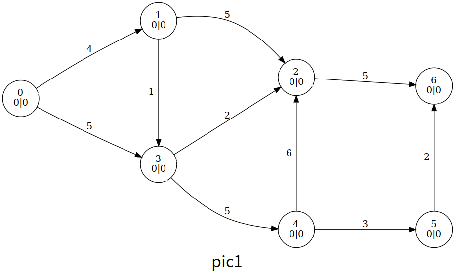
Let's briefly overview the entire algorithm process. Here the author uses a brute-force algorithm, i.e., brute-force scanning for overflowing nodes and updating if found.

Final result:

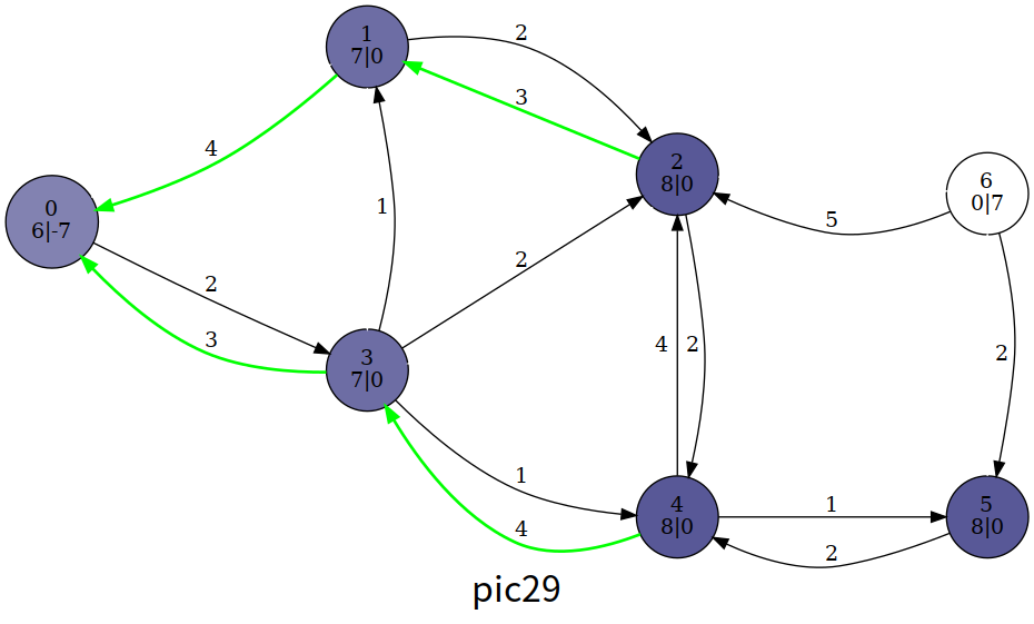
We can see that part of the final excess flow returns to \(s\), and except for source and sink, no other nodes overflow; at this point, the flow function \(f\) satisfies flow conservation and is the maximum flow, with flow value equal to \(e(t)\).

However, actually the paper⁵ points out that only processing overflowing nodes with height less than \(n\) can still obtain the correct maximum flow value. But then at the end of the algorithm, the preflow does not satisfy the flow function properties, and we cannot know the true flow on each edge.

Implementation

Core Code

constexpr int N = 1e4 + 4, M = 1e5 + 5, INF = 0x3f3f3f3f;
int n, m, s, t, maxflow, tot;
int ht[N], ex[N];

void init() {  // initialization
  for (int i = h[s]; i; i = e[i].nex) {
    const int &v = e[i].t;
    ex[v] = e[i].v, ex[s] -= ex[v], e[i ^ 1].v = e[i].v, e[i].v = 0;
  }
  ht[s] = n;
}

bool push(int ed) {
  const int &u = e[ed ^ 1].t, &v = e[ed].t;
  int flow = min(ex[u], e[ed].v);
  ex[u] -= flow, ex[v] += flow, e[ed].v -= flow, e[ed ^ 1].v += flow;
  return ex[u];  // returns 1 if u still overflows
}

void relabel(int u) {
  ht[u] = INF;
  for (int i = h[u]; i; i = e[i].nex)
    if (e[i].v) ht[u] = min(ht[u], ht[e[i].t]);
  ++ht[u];
}

HLPP Algorithm

The Highest Label Preflow Push (HLPP) algorithm, in the generic preflow-push algorithm, always prioritizes selecting the overflowing node with the highest height. Its time complexity is \(O(n^2\sqrt m)\).

Process

Specifically, the HLPP algorithm proceeds as follows:

Initialize (based on the preflow-push algorithm);
Select the overflowing node \(u\) with the highest height, and push on all its pushable edges;
If \(u\) still overflows, relabel it, go back to step 2;
If there are no overflowing nodes, the algorithm ends.

A paper⁶ testing the actual performance of maximum flow algorithms shows that in fact, for preflow-based algorithms, a considerable amount of time is spent on relabeling. Below we introduce two optimizations from the paper⁷ that can significantly reduce the number of relabelings.

BFS Optimization

The upper bound of HLPP is \(O(n^2\sqrt m)\), but it's quite tight in practice. We can optimize when initializing heights. Specifically, we initialize \(h(u)\) as the shortest distance from \(u\) to \(t\); in particular, \(h(s)=n\).

During BFS, we also check graph connectivity to rule out infeasible cases.

GAP Optimization

HLPP pushes when \(h(u)=h(v)+1\). If at some point in the algorithm, there exists some \(k\) such that the number of nodes with \(h(u)=k\) is \(0\), then for nodes with \(h(u)>k\), they can never push excess flow to \(t\), so they can only send it back to \(s\). At that moment, we directly set their height to at least \(n+1\) to quickly push back to \(s\), reducing relabel operations.

The implementation below adopts the method from the paper⁶, using \(N*2-1\) buckets B, where B[i] records all currently overflowing nodes with height \(i\). It incorporates the two optimizations mentioned above and only processes overflowing nodes with height less than \(n\).

It is worth noting that the buckets used in the paper⁶ are linked-list-based stacks, while the default container for stack in STL is deque. Simple tests show that vector, deque, list have little difference in actual running efficiency for this problem.

Implementation

LuoguP4722【Template】Maximum Flow Enhanced Edition/Preflow Push

#include <cstdio>
#include <cstring>
#include <queue>
#include <stack>
using namespace std;
constexpr int N = 1200, M = 120000, INF = 0x3f3f3f3f;
int n, m, s, t;

struct qxx {
  int nex, t;
  long long v;
};

qxx e[M * 2 + 1];
int h[N + 1], cnt = 1;

void add_path(int f, int t, long long v) {
  e[++cnt] = qxx{h[f], t, v}, h[f] = cnt;
}

void add_flow(int f, int t, long long v) {
  add_path(f, t, v);
  add_path(t, f, 0);
}

int ht[N + 1];        // height;
long long ex[N + 1];  // excess flow;
int gap[N];           // gap optimization. gap[i] is the number of nodes with height i
stack<int> B[N];      // bucket B[i] records all v with ht[v]==i
int level = 0;        // highest height among overflowing nodes

int push(int u) {      // push excess flow through pushable edges as much as possible
  bool init = u == s;  // whether initializing
  for (int i = h[u]; i; i = e[i].nex) {
    const int &v = e[i].t;
    const long long &w = e[i].v;
    // during initialization, ignore height difference of 1
    if (!w || (init == false && ht[u] != ht[v] + 1) || ht[v] == INF) continue;
    long long k = init ? w : min(w, ex[u]);
    // take min of residual capacity and excess flow; during initialization, can make source excess negative.
    if (v != s && v != t && !ex[v]) B[ht[v]].push(v), level = max(level, ht[v]);
    ex[u] -= k, ex[v] += k, e[i].v -= k, e[i ^ 1].v += k;  // push
    if (!ex[u]) return 0;  // return if done pushing
  }
  return 1;
}

void relabel(int u) {  // relabel (height)
  ht[u] = INF;
  for (int i = h[u]; i; i = e[i].nex)
    if (e[i].v) ht[u] = min(ht[u], ht[e[i].t]);
  if (++ht[u] < n) {  // only process nodes with height < n
    B[ht[u]].push(u);
    level = max(level, ht[u]);
    ++gap[ht[u]];  // new height, update gap
  }
}

bool bfs_init() {
  memset(ht, 0x3f, sizeof(ht));
  queue<int> q;
  q.push(t), ht[t] = 0;
  while (q.size()) {  // reverse BFS, enqueue unvisited nodes
    int u = q.front();
    q.pop();
    for (int i = h[u]; i; i = e[i].nex) {
      const int &v = e[i].t;
      if (e[i ^ 1].v && ht[v] > ht[u] + 1) ht[v] = ht[u] + 1, q.push(v);
    }
  }
  return ht[s] != INF;  // return 0 if graph disconnected
}

// select one of the nodes with current highest height; return 0 if no overflowing nodes
int select() {
  while (level > -1 && B[level].size() == 0) level--;
  return level == -1 ? 0 : B[level].top();
}

long long hlpp() {            // return maximum flow
  if (!bfs_init()) return 0;  // graph disconnected
  memset(gap, 0, sizeof(gap));
  for (int i = 1; i <= n; i++)
    if (ht[i] != INF) gap[ht[i]]++;  // initialize gap
  ht[s] = n;
  push(s);  // initialize preflow
  int u;
  while ((u = select())) {
    B[level].pop();
    if (push(u)) {  // still overflowing
      if (!--gap[ht[u]])
        for (int i = 1; i <= n; i++)
          if (i != s && ht[i] > ht[u] && ht[i] < n + 1)
            ht[i] = n + 1;  // nodes relabeled to n+1 here are not overflowing
      relabel(u);
    }
  }
  return ex[t];
}

int main() {
  scanf("%d%d%d%d", &n, &m, &s, &t);
  for (int i = 1, u, v, w; i <= m; i++) {
    scanf("%d%d%d", &u, &v, &w);
    add_flow(u, v, w);
  }
  printf("%lld", hlpp());
  return 0;
}

Experience the running process:

HLPP

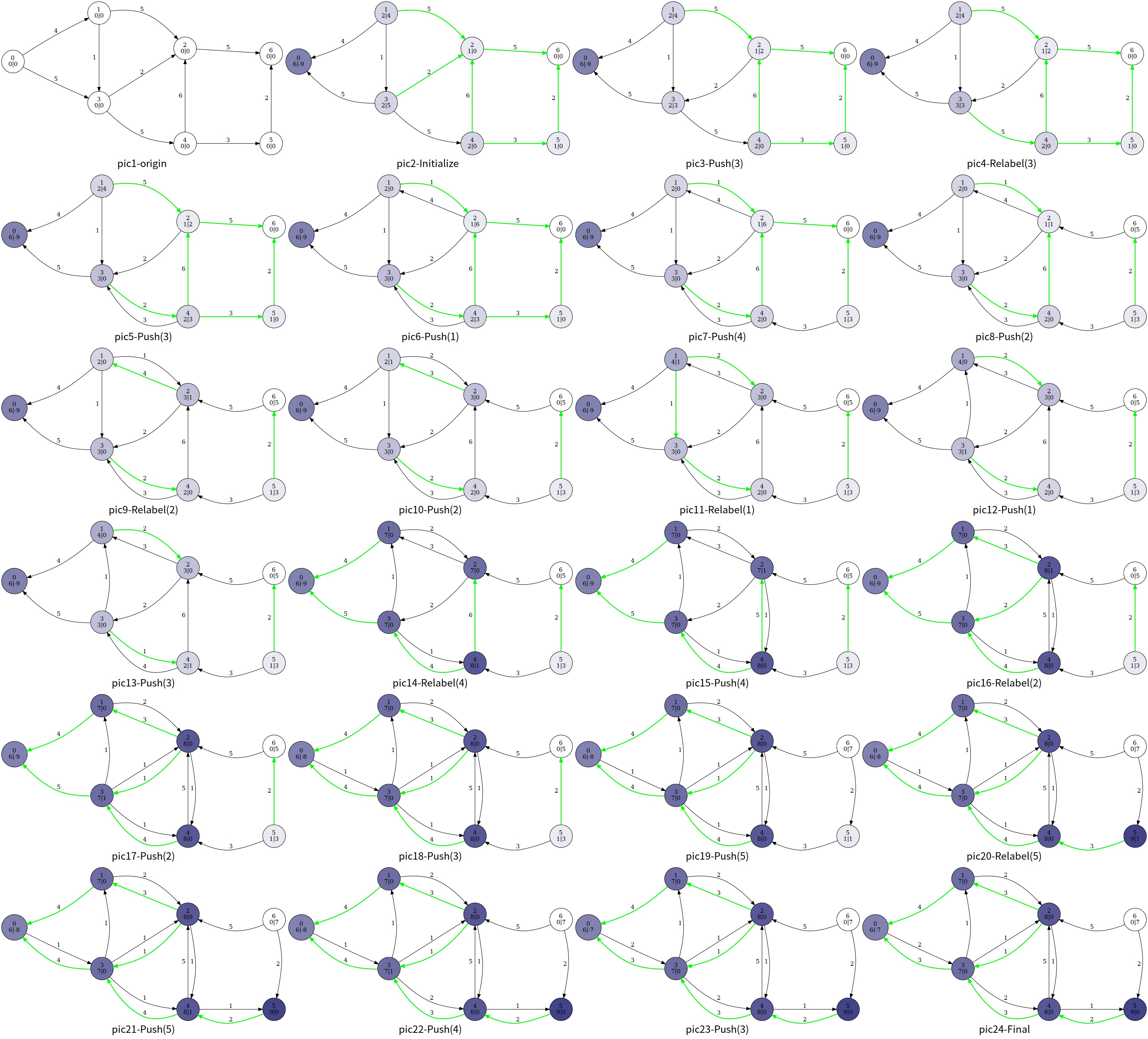
Between pic13 and pic14, Relabel(4) is executed, and GAP optimization is performed.

Footnotes

http://pisces.ck.tp.edu.tw/~peng/index.php?action=showfile&file=f6cdf7ef750d7dc79c7d599b942acbaaee86a2e3e ↩
https://people.orie.cornell.edu/dpw/orie633/LectureNotes/lecture9.pdf ↩
In English literature, usually called "active". ↩
In English literature, a node's height is often called "distance label". The term "height" used here comes from relevant chapters in Introduction to Algorithms. You can find the reason for doing so in footnote on P432 of the Mechanical Industry Press edition of Introduction to Algorithms (Original 3^rd Edition). ↩
Cherkassky B V, Goldberg A V. On implementing push-relabel method for the maximum flow problem[C]//International Conference on Integer Programming and Combinatorial Optimization. Springer, Berlin, Heidelberg, 1995: 157-171. ↩
Ahuja R K, Kodialam M, Mishra A K, et al. Computational investigations of maximum flow algorithms[J]. European Journal of Operational Research, 1997, 97(3): 509-542. ↩↩↩
Derigs U, Meier W. Implementing Goldberg's max-flow-algorithm—A computational investigation[J]. Zeitschrift für Operations Research, 1989, 33(6): 383-403. ↩

本页面最近更新：，更新历史
发现错误？想一起完善？在 GitHub 上编辑此页！
本页面贡献者：OI-wiki
本页面的全部内容在 CC BY-SA 4.0 和 SATA 协议之条款下提供，附加条款亦可能应用

Maximum Flow

Overview

Ford–Fulkerson Augmentation

Overview

Max-Flow Min-Cut Theorem

Time Complexity Analysis

Edmonds–Karp Algorithm

Algorithm Idea

Time Complexity Analysis

Code Implementation

Dinic Algorithm

Algorithm Idea

Time Complexity Analysis

Time Complexity Analysis in Special Cases

Code Implementation

MPM Algorithm

Time Complexity Analysis

Implementation

ISAP

Process

Implementation

Push-Relabel Preflow-Push Algorithm

Generic Preflow-Push Algorithm

Height Function4

Push

Relabel

Initialization

Process

Implementation

HLPP Algorithm

Process

BFS Optimization

GAP Optimization

Implementation

Footnotes

Height Function⁴