Dancing Links
This page introduces the Exact Cover Problem, the Repeated Cover Problem, the algorithm "Algorithm X" to solve these problems, and the Dancing Links (DLX) data structure used to optimize Algorithm X. This page also explains how to use DLX with modeling to solve some search problems.
Exact Cover Problem
Definition
The Exact Cover Problem is defined as: given many sets \(S_i (1 \le i \le n)\) and a set \(X\), find an unordered multiset \((T_1, T_2, \cdots , T_m)\) satisfying the following conditions:
- \(\forall i, j \in [1, m],T_i\bigcap T_j = \varnothing (i \neq j)\)
- \(X = \bigcup\limits_{i = 1}^{m}T_i\)
- \(\forall i \in[1, m], T_i \in \{S_1, S_2, \cdots, S_n\}\)
Explanation
For example, given
then \((S_1, S_4, S_5)\) is a valid solution.
Problem Transformation
Discretize all numbers in \(\bigcup\limits_{i = 1}^{n}S_i\) to obtain the following model:
Given a 0-1 matrix, you can select some rows such that eventually each column1 has exactly one 1. For example, modeling the above example yields the following matrix:
Here, row \(i\) represents \(S_i\), and each number in this row indicates \([1 \in S_i],[3 \in S_i],[5 \in S_i],\cdots,[119 \in S_i]\) in order.
Implementation
Brute Force 1
One method is to enumerate which rows are selected, then check if the selection is valid.
Since each row can be either selected or not, enumerating rows has time complexity \(O(2^n)\);
Each check requires \(O(nm)\) time. So the total complexity is \(O(nm\cdot2^n)\).
Implementation
1 2 3 4 5 6 7 8 9 10 11 12 13 14 15 16 17 18 19 20 21 22 23 24 25 | |
Brute Force 2
Considering the special property of the 0-1 matrix, each row can be viewed as an \(m\)-bit binary number.
Thus the original problem transforms into:
Given \(n\) \(m\)-bit binary numbers, select some numbers such that the bitwise AND of any two numbers is 0, and the bitwise OR of all selected numbers is \(2^m - 1\).
tmprepresents the bitwise OR of the currently selected binary numbers.
Since each row has two states (selected or not), enumerating rows has time complexity \(O(2^n)\);
Each computation of tmp requires \(O(n)\) time. So the total complexity is \(O(n\cdot2^n)\).
Implementation
1 2 3 4 5 6 7 8 9 10 11 12 13 14 15 16 17 18 19 20 21 22 | |
Repeated Cover Problem
The Repeated Cover Problem is similar to the Exact Cover Problem, but without the restriction on element uniqueness. The Algorithm X introduced below was originally designed for the Exact Cover Problem, but with some modifications and optimizations (noted within), it can also efficiently solve the Repeated Cover Problem.
Algorithm X
Donald E. Knuth proposed Algorithm X, whose idea is similar to the brute-force approach above but is more convenient to optimize.
Process
Continuing with the example mentioned earlier, we obtain the following 0-1 matrix:
-
Currently, row 1 has \(3\) ones, row 2 has \(3\) ones, row 3 has \(3\) ones, row 4 has \(2\) ones, row 5 has \(2\) ones, row 6 has \(3\) ones. Select row 1, delete it, and mark all columns containing a 1 in this row;
\[ \begin{pmatrix} \color{Blue}0 & \color{Blue}0 & \color{Blue}1 & \color{Blue}0 & \color{Blue}1 & \color{Blue}1 & \color{Blue}0 \\ 1 & 0 & \color{Red}0 & 1 & \color{Red}0 & \color{Red}0 & 1 \\ 0 & 1 & \color{Red}1 & 0 & \color{Red}0 & \color{Red}1 & 0 \\ 1 & 0 & \color{Red}0 & 1 & \color{Red}0 & \color{Red}0 & 0 \\ 0 & 1 & \color{Red}0 & 0 & \color{Red}0 & \color{Red}0 & 1 \\ 0 & 0 & \color{Red}0 & 1 & \color{Red}1 & \color{Red}0 & 1 \end{pmatrix} \] -
Select all marked columns, delete them, and mark all rows containing a 1 in these columns (for the Repeated Cover Problem, marking is not necessary);
\[ \begin{pmatrix} \color{Blue}0 & \color{Blue}0 & \color{Blue}1 & \color{Blue}0 & \color{Blue}1 & \color{Blue}1 & \color{Blue}0 \\ 1 & 0 & \color{Blue}0 & 1 & \color{Blue}0 & \color{Blue}0 & 1 \\ \color{Red}0 & \color{Red}1 & \color{Blue}1 & \color{Red}0 & \color{Blue}0 & \color{Blue}1 & \color{Red}0 \\ 1 & 0 & \color{Blue}0 & 1 & \color{Blue}0 & \color{Blue}0 & 0 \\ 0 & 1 & \color{Blue}0 & 0 & \color{Blue}0 & \color{Blue}0 & 1 \\ \color{Red}0 & \color{Red}0 & \color{Blue}0 & \color{Red}1 & \color{Blue}1 & \color{Blue}0 & \color{Red}1 \end{pmatrix} \] -
Select all marked rows and delete them;
\[ \begin{pmatrix} \color{Blue}0 & \color{Blue}0 & \color{Blue}1 & \color{Blue}0 & \color{Blue}1 & \color{Blue}1 & \color{Blue}0 \\ 1 & 0 & \color{Blue}0 & 1 & \color{Blue}0 & \color{Blue}0 & 1 \\ \color{Blue}0 & \color{Blue}1 & \color{Blue}1 & \color{Blue}0 & \color{Blue}0 & \color{Blue}1 & \color{Blue}0 \\ 1 & 0 & \color{Blue}0 & 1 & \color{Blue}0 & \color{Blue}0 & 0 \\ 0 & 1 & \color{Blue}0 & 0 & \color{Blue}0 & \color{Blue}0 & 1 \\ \color{Blue}0 & \color{Blue}0 & \color{Blue}0 & \color{Blue}1 & \color{Blue}1 & \color{Blue}0 & \color{Blue}1 \end{pmatrix} \]This indicates that this row has been selected, and no other 1s are allowed in the columns where this row has 1s.
Thus we obtain a new small 0-1 matrix:
\[ \begin{pmatrix} 1 & 0 & 1 & 1 \\ 1 & 0 & 1 & 0 \\ 0 & 1 & 0 & 1 \end{pmatrix} \] -
Now row 1 (originally row 2) has \(3\) ones, row 2 (originally row 4) has \(2\) ones, row 3 (originally row 5) has \(2\) ones. Select row 1 (originally row 2), delete it, and mark all columns containing a 1 in this row;
\[ \begin{pmatrix} \color{Blue}1 & \color{Blue}0 & \color{Blue}1 & \color{Blue}1 \\ \color{Red}1 & 0 & \color{Red}1 & \color{Red}0 \\ \color{Red}0 & 1 & \color{Red}0 & \color{Red}1 \end{pmatrix} \] -
Select all marked columns, delete them, and mark all rows containing a 1 in these columns;
\[ \begin{pmatrix} \color{Blue}1 & \color{Blue}0 & \color{Blue}1 & \color{Blue}1 \\ \color{Blue}1 & \color{Red}0 & \color{Blue}1 & \color{Blue}0 \\ \color{Blue}0 & \color{Red}1 & \color{Blue}0 & \color{Blue}1 \end{pmatrix} \] -
Select all marked rows and delete them;
\[ \begin{pmatrix} \color{Blue}1 & \color{Blue}0 & \color{Blue}1 & \color{Blue}1 \\ \color{Blue}1 & \color{Blue}0 & \color{Blue}1 & \color{Blue}0 \\ \color{Blue}0 & \color{Blue}1 & \color{Blue}0 & \color{Blue}1 \end{pmatrix} \]This yields an empty matrix. However, the last deleted row
1 0 1 1is not all ones, indicating an incorrect selection;\[ \begin{pmatrix} \end{pmatrix} \] -
Backtrack to step 4, consider selecting row 2 (originally row 4), delete it, and mark all columns containing a 1 in this row;
\[ \begin{pmatrix} \color{Red}1 & 0 & \color{Red}1 & 1 \\ \color{Blue}1 & \color{Blue}0 & \color{Blue}1 & \color{Blue}0 \\ \color{Red}0 & 1 & \color{Red}0 & 1 \end{pmatrix} \] -
Select all marked columns, delete them, and mark all rows containing a 1 in these columns;
\[ \begin{pmatrix} \color{Blue}1 & \color{Red}0 & \color{Blue}1 & \color{Red}1 \\ \color{Blue}1 & \color{Blue}0 & \color{Blue}1 & \color{Blue}0 \\ \color{Blue}0 & 1 & \color{Blue}0 & 1 \end{pmatrix} \] -
Select all marked rows and delete them;
\[ \begin{pmatrix} \color{Blue}1 & \color{Blue}0 & \color{Blue}1 & \color{Blue}1 \\ \color{Blue}1 & \color{Blue}0 & \color{Blue}1 & \color{Blue}0 \\ \color{Blue}0 & 1 & \color{Blue}0 & 1 \end{pmatrix} \]Thus we obtain the following matrix:
\[ \begin{pmatrix} 1 & 1 \end{pmatrix} \] -
Now row 1 (originally row 5) has \(2\) ones, delete them all, yielding an empty matrix:
\[ \begin{pmatrix} \end{pmatrix} \] -
The last deletion removed a row that was all ones, so the algorithm succeeds and terminates.
The answer is the three deleted rows: \(1, 4, 5\).
It is highly recommended to simulate the matrix deletion, restoration, and backtracking process yourself before continuing.
Through the above steps, the process of Algorithm X can be summarized as follows:
- For the current matrix \(M\), select and mark a row \(r\), add \(r\) to \(S\);
- If all \(r\) have been tried without a solution, the algorithm terminates, outputting no solution;
- Mark the rows \(r_i\) and columns \(c_i\) related to \(r\) (the definition of related rows and columns is the same as in step 2 of Algorithm X, similarly below);
- Delete all marked rows and columns, obtaining a new matrix \(M'\);
-
If \(M'\) is empty and \(r\) is all ones, the algorithm terminates, outputting the set \(S\) of deleted rows;
If \(M'\) is empty and \(r\) is not all ones, restore the rows \(r_i\) and columns \(c_i\) related to \(r\), jump to step 1;
If \(M'\) is not empty, jump to step 1.
It is not hard to see that Algorithm X requires many "delete row", "delete column", "restore row", and "restore column" operations.
A naive idea is to use a two-dimensional array to store the matrix, and four arrays to store the adjacent row numbers for each row, updating only the elements in these four arrays during deletion and restoration. However, since the number of 0s in typical problem matrices far exceeds the number of 1s, the space complexity of this approach is unacceptable.
Donald E. Knuth thought of using a doubly linked cross list (Dancing Links) to maintain these operations.
The process of continuously jumping on the doubly linked cross list is vividly compared to "dancing", hence the doubly linked cross list used to optimize Algorithm X is also called "Dancing Links".
Dancing Links Optimized Algorithm X
Preprocessor Macro
1 | |
Definition
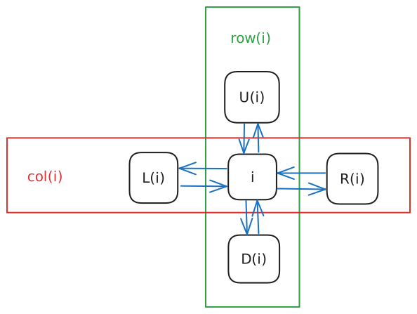
Each node in the doubly linked cross list has four pointer fields, pointing to the up, down, left, and right elements; and each element \(i\) corresponds to a cell in the entire doubly linked cross list system, so it also needs to represent the column and row where \(i\) is located, as shown in the figure:
A large doubly linked cross list is more complex:
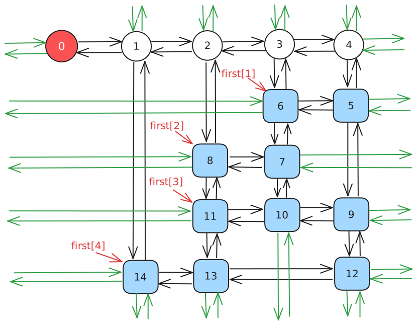
Each row has a row head indicator, and each column has a column indicator.
The row head indicator is first[], and the column indicators are \(c + 1\) newly created sentinel nodes. Notably, the row head indicator is not a sentinel node in the linked list. It is virtual, similar to the first[] array in adjacency lists, directly pointing to the first element in that row.
Also, each column has a siz[] indicating the number of elements in that column.
Specifically, node \(0\) having no right node is equivalent to the Dancing Links being empty.
1 2 3 4 | |
Process
remove Operation
remove(c) means deleting column \(c\) and its related rows and columns from the Dancing Links.
First delete \(c\), at this point:
- The right node of the node to the left of \(c\) should be the right node of \(c\).
- The left node of the node to the right of \(c\) should be the left node of \(c\).
That is L[R[c]] = L[c], R[L[c]] = R[c];.
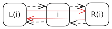
Then go down this column, deleting each row encountered.
How to delete each row? Enumerate the pointer \(j\) of the current row, at this point:
- The down node of the node above \(j\) should be the down node of \(j\).
- The up node of the node below \(j\) should be the up node of \(j\).
Note to modify the element count for each column.
That is U[D[j]] = U[j], D[U[j]] = D[j], --siz[col[j]];.
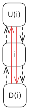
The code implementation of the remove function is as follows:
Implementation
1 2 3 4 5 6 7 8 9 | |
recover Operation
recover(c) means restoring column \(c\) and its related rows and columns in the Dancing Links.
recover(c) is the inverse operation of remove(c), and will not be elaborated here.
It is worth noting that the order of all operations in recover(c) is exactly the opposite of the operations in remove(c).
The code implementation of recover(c) is as follows:
Implementation
1 2 3 4 5 | |
build Operation
build(r, c) means creating a new Dancing Links of size \(r \times c\), i.e., with \(r\) rows and \(c\) columns.
Create \(c + 1\) nodes as column indicators.
The left node of the \(i\)-th node is \(i - 1\), the right node is \(i + 1\), the up node is \(i\), and the down node is \(i\). Specifically, the left node of node \(0\) is \(c\), and the right node of node \(c\) is \(0\).
Thus we obtain a circular doubly linked list:
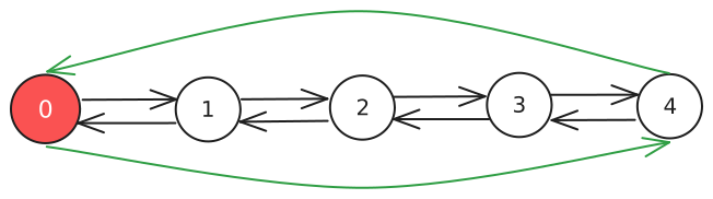
This initializes a Dancing Links.
The code implementation of build(r, c) is as follows:
Implementation
1 2 3 4 5 6 7 8 9 10 | |
insert Operation
insert(r, c) means inserting a node at row \(r\), column \(c\).
The insertion operation is divided into two cases:
-
If row \(r\) has no elements, then directly insert an element and make
first[r]point to this element.This can be achieved by
first[r] = L[idx] = R[idx] = idx;. -
If row \(r\) has elements, then connect this new element to \(c\) and \(first(r)\) in a special way.
Let this new element be \(idx\), then:
-
Insert \(idx\) directly below \(c\), at this point:
- The down node of \(idx\) is the original down node of \(c\);
- The up node of the node below \(idx\) (i.e., the original down node of \(c\)) is \(idx\);
- The up node of \(idx\) is \(c\);
- The down node of \(c\) is \(idx\).
Note to record the column and row of \(idx\), and update the element count of this column.
1
2
col[++idx] = c, row[idx] = r, ++siz[c];
U[idx] = c, D[idx] = D[c], U[D[c]] = idx, D[c] = idx;
It is strongly recommended that readers fully grasp the order of these steps before continuing.
-
Insert \(idx\) directly to the right of \(first(r)\), at this point:
- The right node of \(idx\) is the original right node of \(first(r)\);
- The left node of the original right node of \(first(r)\) is \(idx\);
- The left node of \(idx\) is \(first(r)\);
- The right node of \(first(r)\) is \(idx\).
1
2
L[idx] = first[r], R[idx] = R[first[r]];
L[R[first[r]]] = idx, R[first[r]] = idx;
It is strongly recommended that readers fully grasp the order of these steps before continuing.
-
The insert(r, c) operation can be understood with the aid of the following image:
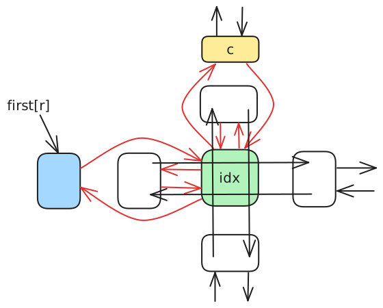
Pay attention to the direction of the curved arrows.
The code implementation of insert(r, c) is as follows:
Implementation
1 2 3 4 5 6 7 8 9 10 | |
dance Operation
dance() is the process of recursively deleting and restoring various rows and columns.
- If node \(0\) has no right node, then the matrix is empty, record the answer and return;
- Select the column with the fewest elements and delete this column;
- Traverse all rows with a 1 in this column, enumerate whether it is selected;
- Recursively call
dance(); if feasible, return; if not feasible, restore the selected row; - If no solution, return.
The code implementation of dance() is as follows:
Implementation
1 2 3 4 5 6 7 8 9 10 11 12 13 14 15 16 17 | |
Here stk[] is used to record the answer.
Note that we always prioritize selecting the column with the fewest elements for deletion, which ensures the algorithm has some heuristic, minimizing the search tree branches.
For the Repeated Cover Problem, a heuristic function (similar to A*) can be used for pruning during search: if the current best-case number of selected rows exceeds the current optimal solution, return directly.
Template
Template Code
1 2 3 4 5 6 7 8 9 10 11 12 13 14 15 16 17 18 19 20 21 22 23 24 25 26 27 28 29 30 31 32 33 34 35 36 37 38 39 40 41 42 43 44 45 46 47 48 49 50 51 52 53 54 55 56 57 58 59 60 61 62 63 64 65 66 67 68 69 70 71 72 73 74 75 76 77 78 79 80 81 82 83 84 85 86 87 88 89 90 | |
Properties
The number of recursions and backtracks in DLX is related to the number of 1s in the matrix, not to parameters like \(r, c\) of the matrix. Therefore, its time complexity is exponential, theoretically around \(O(c^n)\), where \(c\) is some constant very close to 1, and \(n\) is the number of 1s in the matrix.
But in practice, DLX performs well and can generally solve most problems.
Modeling
The difficulty of DLX lies not only in building the linked list but also in modeling.
Please ensure you have fully mastered the DLX template before continuing.
For each problem we encounter, we should consider the meaning of rows and columns:
-
Rows represent decisions, because each row corresponds to a set, i.e., to select or not select;
-
Columns represent states, because column \(i\) corresponds to some condition \(P_i\).
For a given row, since the values in different columns vary, we define a decision by different states.
Example 1 P1784 Sudoku
Solution Idea
First consider what a decision is.
In this problem, each decision can be represented by an ordered triple \((r, c, w)\).
Note that the "box" is not a parameter of the decision because it can be represented by each determined \((r, c)\).
Therefore there are \(9 \times 9 \times 9 = 729\) rows.
Then consider what a state is.
Think about what effect the decision \((r, c, w)\) will cause. Let the box containing \((r, c)\) be \(b\).
- Row \(r\) uses a \(w\) (represented by \(9 \times 9 = 81\) columns);
- Column \(c\) uses a \(w\) (represented by \(9 \times 9 = 81\) columns);
- Box \(b\) uses a \(w\) (represented by \(9 \times 9 = 81\) columns);
- Cell \((r, c)\) is filled with a number (represented by \(9 \times 9 = 81\) columns).
Therefore there are \(81 \times 4 = 324\) columns, totaling \(729 \times 4 = 2916\) ones.
Thus, we have successfully transformed the \(9 \times 9\) Sudoku problem into an exact cover problem with \(729\) rows, \(324\) columns, and \(2916\) ones.
Reference Code
1 2 3 4 5 6 7 8 9 10 11 12 13 14 15 16 17 18 19 20 21 22 23 24 25 26 27 28 29 30 31 32 33 34 35 36 37 38 39 40 41 42 43 44 45 46 47 48 49 50 51 52 53 54 55 56 57 58 59 60 61 62 63 64 65 66 67 68 69 70 71 72 73 74 75 76 77 78 79 80 81 82 83 84 85 86 87 88 89 90 91 92 93 94 95 96 97 98 99 100 101 102 103 104 105 106 107 108 109 110 111 112 | |
Example 2 Target Sudoku
Solution Idea
The model construction for this problem is exactly the same as for Sudoku, the main difference lies in updating the answer.
For this problem, we can maintain a weight array. Each time a Sudoku solution is found,
multiply the number in each position by the corresponding weight and add to the answer.
Reference Code
1 2 3 4 5 6 7 8 9 10 11 12 13 14 15 16 17 18 19 20 21 22 23 24 25 26 27 28 29 30 31 32 33 34 35 36 37 38 39 40 41 42 43 44 45 46 47 48 49 50 51 52 53 54 55 56 57 58 59 60 61 62 63 64 65 66 67 68 69 70 71 72 73 74 75 76 77 78 79 80 81 82 83 84 85 86 87 88 89 90 91 92 93 94 95 96 97 98 99 100 101 102 103 104 105 106 107 108 109 110 111 112 113 114 115 116 117 118 119 120 121 122 123 | |
Example 3 「NOI2005」Wisdom Pearl Game
Solution Idea
Definition: The shape of a wisdom pearl given in the problem is called its standard shape.
Obviously, we can change the shape of a wisdom pearl by varying two parameters \(d\) (number of clockwise \(90^{\circ}\) rotations) and \(f\) (whether to flip horizontally).
Again, first consider what a decision is.
In this problem, each decision can be represented by an ordered quintuple \((v, d, f, i)\).
It means placing the top-left corner of the standard shape of the \(i\)-th wisdom pearl at position \(v\), after \(d\) clockwise rotations of \(90^{\circ}\).
Coincidentally, we can set \(f = 1\) for no horizontal flip and \(f = -1\) for horizontal flip, simplifying the code.
Therefore there are \(55 \times 4 \times 2 \times 12 = 5280\) rows.
Note that due to some illegal placements, such as \((1, 0, 1, 4)\),
in practice, the empty wisdom pearl board only needs to generate \(2730\) rows.
Then consider what a state is.
The state in this problem is relatively simple.
Think about what effect the decision \((v, d, f, i)\) will cause.
- Certain cells are occupied (represented by \(55\) columns);
- The \(i\)-th wisdom pearl is used (represented by \(12\) columns).
Therefore there are \(55 + 12 = 67\) columns, totaling \(5280 \times (5 + 1) = 31680\) ones.
Thus, we have successfully transformed the Wisdom Pearl Game into an exact cover problem with \(5280\) rows, \(67\) columns, and \(31680\) ones.
Reference Code
1 2 3 4 5 6 7 8 9 10 11 12 13 14 15 16 17 18 19 20 21 22 23 24 25 26 27 28 29 30 31 32 33 34 35 36 37 38 39 40 41 42 43 44 45 46 47 48 49 50 51 52 53 54 55 56 57 58 59 60 61 62 63 64 65 66 67 68 69 70 71 72 73 74 75 76 77 78 79 80 81 82 83 84 85 86 87 88 89 90 91 92 93 94 95 96 97 98 99 100 101 102 103 104 105 106 107 108 109 110 111 112 113 114 115 116 117 118 119 120 121 122 123 124 125 126 127 128 129 130 131 132 133 134 135 136 137 138 139 140 141 142 143 144 145 146 147 148 149 150 151 152 153 154 155 156 157 158 159 160 161 162 163 164 165 166 167 168 169 | |
Exercises
External Links
- Dancing Links Algorithm for Exact Cover Problem - 万仓一黍
- Search: DLX Algorithm - 静听风吟。
- 《Algorithm Competition Introduction Classic - Training Guide》
Notes
-
(Terminology difference across the strait) Taiwan: column (直行), row (橫列). ↩
本页面最近更新:,更新历史
发现错误?想一起完善? 在 GitHub 上编辑此页!
本页面贡献者:OI-wiki
本页面的全部内容在 CC BY-SA 4.0 和 SATA 协议之条款下提供,附加条款亦可能应用